7  Results at a glance

The next nine chapters report what the 7,200 fits showed. This one states the results in compressed form, so that a reader who goes no further leaves with the study’s answer, and so that the detailed chapters can be read against a map of where they are going. We begin with the check that has to come first: whether the comparison machinery can be trusted at all.

7.1 The calibration control, before anything else

The design reserves its forty normal-population cells as a negative control. On those cells the Gaussian prior is correctly specified, so the flexible prior has nothing legitimate to win; any win rate much above zero would say that the comparison machinery produces spurious advantages, and the locked plan (Section 6.5) treats that as a blocking alarm for every claim in the study. The realized win rate is 0.0: none of the 40 normal cells produced a win or strong-win label, against a preregistered ceiling of 0.05. The one-sample control contrast estimates the mean log loss ratio on normal cells at +0.016 (95% CI [0.002, 0.030]), a resolvably positive but small quantity: flexible-prior KS loss is about 1.6 percent higher where the Gaussian model is correctly specified. The realized operating characteristic tells the same story from the other side, with type-I rates of 0.035 to 0.048 against the nominal 0.05 (Section 14.3). The gate passed, and the rest of Part III stands on it.

7.2 The two maps that carry the story

Figure 7.1 is the study in one display. For each of the 120 conditions it names the prior + summary combination with the smallest condition-mean loss, once for the distribution-recovery goal and once for the individual-accuracy goal.

Figure 7.1: In this six-combination census, the goal almost always selects the summary while the winning prior varies by regime. Each tile shows the prior + summary combination with the smallest condition-mean loss among the six main combinations (Gaussian or focused DP prior, crossed with the PM, CB and GR summaries), for the distribution-recovery goal in panel (a) and the individual-accuracy goal in panel (b). Tile color gives the winning prior; the glyph gives the winning summary (circle PM, triangle CB, square GR). Opacity is an overall six-combination winner-margin screen: full color means the observed winner leads its runner-up by more than twice the form-paired MCSE of their log-loss difference. The runner-up can share the same prior, so opacity is not a prior-uncertainty key; the post-selection 2 × MCSE rule is descriptive, not a formal 95% interval. Washed cells have smaller observed margins, not necessarily coin-flip winners. Each condition mean averages 20 replications (5 forms x 4 draws). GR wins panel (a) in 113 of 120 cells and PM wins panel (b) in 116 of 120. In an exploratory exhaustive resampling of the five observed form positions, summary identity is stable in 96.7% and 98.8% of cell-resamples, respectively; the expected counts are 112.7 (SD 1.4) and 115.1 (SD 1.2). This conditional stability check supports the census but does not turn the descriptive tiles into family-controlled tests.

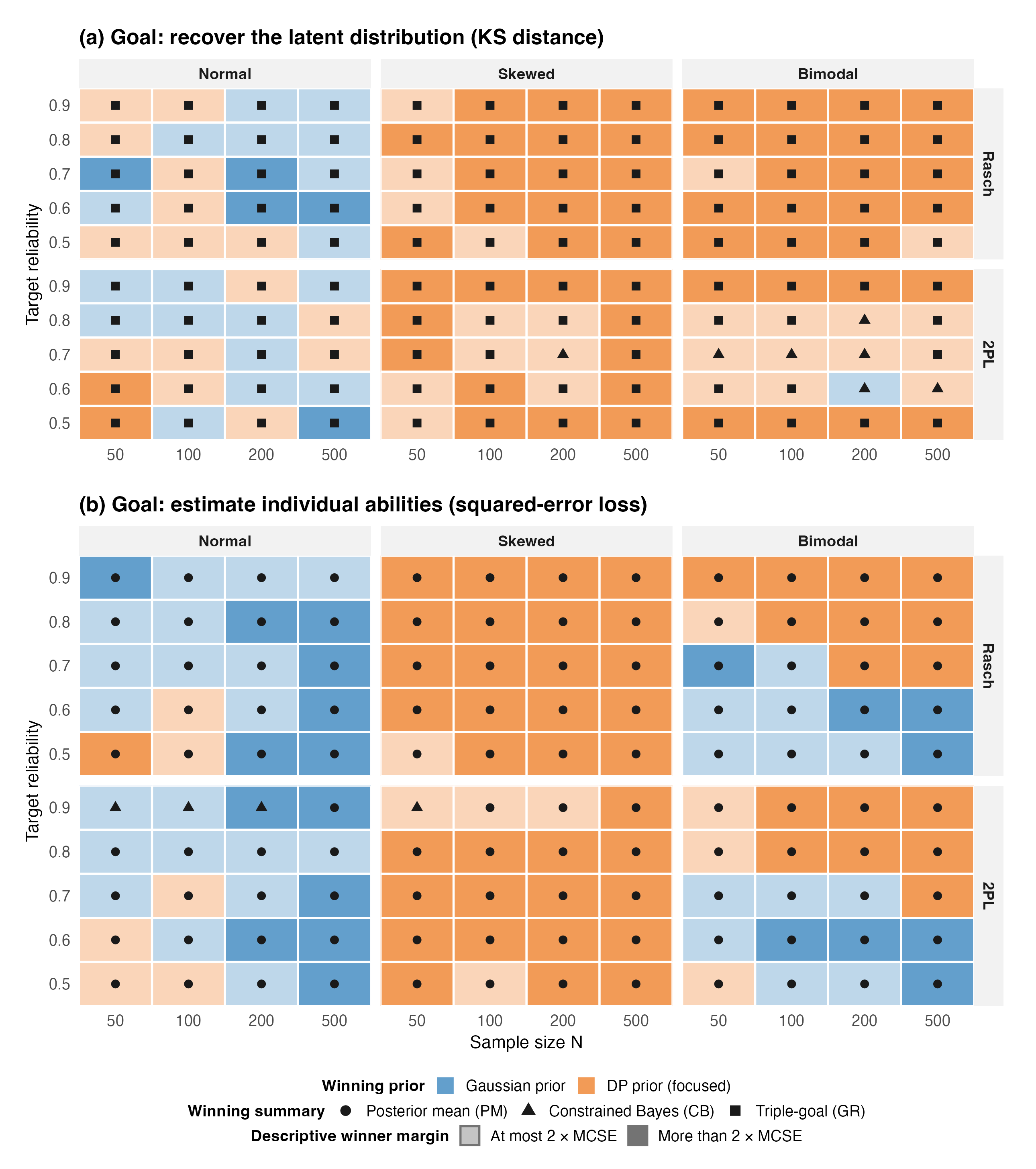
Two regularities organize this exploratory winner census, and they are the study’s storyline. The opacity key is a descriptive stability screen for the margin between the best and runner-up combinations, not a formal interval or a measure of prior uncertainty. The first is that the summary row is decided by the goal. The GR summary wins the distribution-recovery panel in 113 of 120 cells regardless of the prior, and the posterior mean wins the individual-accuracy panel in 116 of 120. Conditional resampling of the five observed form positions retains those summary identities in 96.7% and 98.8% of cell-resamples. Whatever else varies, choosing the summary to match the inferential goal is highly stable in this design. The second is that the prior row is decided by the regime. The flexible prior’s tiles concentrate where non-normality meets information (large N, high reliability), fade toward parity as information falls, and never earn a decisive win under normality. The prior question therefore has no single answer; it has a map, and reliability is one of its two axes.

The magnitude behind the tiles is given by Figure 8.2 in Chapter 8, whose headline numbers are worth carrying: over the non-normal cells the preregistered primary contrast (DP focused + GR against Gaussian + GR) reduces KS loss by a factor of .80 at the design’s center (H1), the reduction deepens by a factor of .89 with each doubling of N (H2), and over the preregistered opportunity region the mean ratio is .73, a 27 percent reduction.

7.3 The result in four sentences

First, the flexible prior improves distribution recovery under non-normality, most strongly where reliability and sample size are high; normal controls mostly cluster near parity but include three cells with a resolved increase in flexible-prior KS loss (H1, H2, H6, calibration control). Second, the posterior summary is the larger lever: swapping the summary moves distributional loss several times more than swapping the prior in most of the grid, and a Gaussian prior with the right summary beats a flexible prior with the wrong one in 100 of 120 cells (H7 and Chapter 9). Third, reliability helps organize the recipe: in most lower-tier cells the prior moves loss less than the summary, although the crossed map retains 2PL skew exceptions at reliability 0.6; at 0.8 and above, under non-normality, the two levers often compound, and the flexible prior with GR is generally the best observed combination (Chapter 10). Fourth, the cross-goal tradeoff is patterned rather than absent: 48 cells improve distribution loss while worsening individual loss, and the H4 safety flags isolate seven bimodal reliability-0.5/0.6 cells with 5 to 14 percent higher MSEL, ratios 1.052 to 1.138, every interval excluding 1 (full cell-level table and post-outcome timing in Section 12.1). For rank loss, differences among the six plotted estimators are small relative to the reliability gradient in this design (H4, Chapter 12, Chapter 13).

7.4 Health of the evidence

Every one of the 7,200 fits entered the analysis: none was excluded, 0 crossed the hard convergence boundary, and 186 (2.6%) carried a soft R-hat warning, with the median across fits of the maximum rank-normalized split R-hat at 1.00314. All six preregistered contrasts met their replication-adequacy targets, so no claim wording is downgraded on precision grounds. Chapter Chapter 14 reports the full record, including the one preregistered sensitivity in which a conclusion visibly weakens (H5 under strict-pass estimation).

7.5 How to read Part III

The chapters that follow are organized by question rather than by hypothesis number. Chapter 8 establishes where the flexible prior improves distribution recovery and what the harm-flag labels do and do not mean. Chapter 9 quantifies the summary-versus-prior comparison and tests it beyond the preregistered family. Chapter 10 puts reliability at the center and extracts the practical recipes. Chapter 11 compares the Rasch and 2PL families. Chapter 12 examines the individual-accuracy tradeoff and gives the seven flagged cells’ complete intervals and Addendum 006’s post-outcome timing. Chapter 13 covers the goals with comparatively small estimator differences. Chapter 14 carries diagnostics, sensitivity analyses and the realized operating characteristic, and Chapter 15 collects the formal preregistered record in one place. Hypothesis tests are reported where their content belongs; the record chapter holds the complete family tables.