| Factor | Levels | Role |
|---|---|---|
| IRT model family | Rasch; 2PL | crossed, co-primary |
| Latent shape | normal (control); skewed (k = 2.0); bimodal (delta = 0.90) | crossed |
| Target reliability | 0.5, 0.6, 0.7, 0.8, 0.9 (nested length + cell-specific c_star calibration) | crossed |
| Sample size N | 50, 100, 200, 500 | crossed |
| Fitted prior | Gaussian; DP focused; DP broad | within dataset |
| Posterior summary | PM; CB; GR (from the same fit) | within fit |
| Form replicate | 5 independent item banks per condition | replication |
| Response draw | 4 per form (20 datasets per condition) | replication |
| Source: frozen production design as summarized in the generated F$design component; the reliability ladder uses the design's nested-length, cell-specific c_star calibration. | ||
4 The design
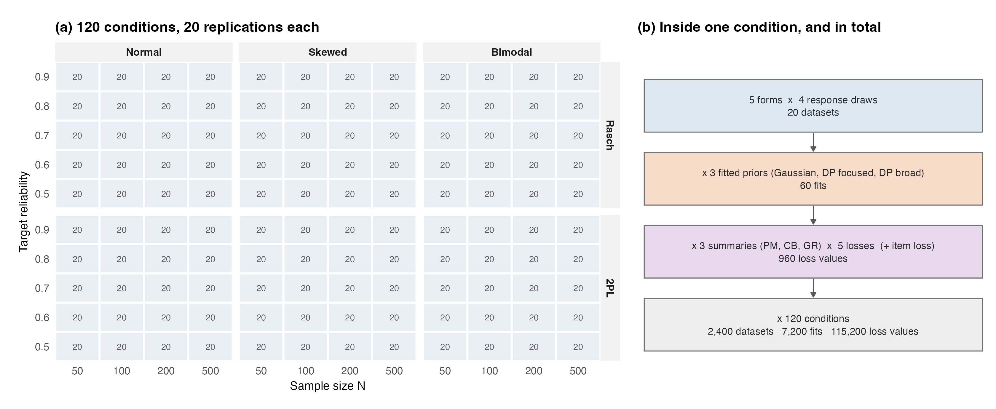
The design crosses everything that the argument of Part I says must be crossed: model family, latent shape, reliability, sample size, prior, and summary. This chapter walks the grid, the replication structure inside each condition, and the two disclosed asymmetries that reliability-matching between families produces. Here reliability matching means the actual nested-length plus global-scale calibration, not length matching alone. Figure 4.1 shows the whole at a glance.
4.1 Factors and their levels
The table’s compact reliability label denotes the full frozen construction. Item count rises through a nested ladder, and a multiplier \(c^\star\) is then calibrated and applied separately for each model, form, tier and latent shape. There are 150 such calibration cells. Test length is constant across shapes within a model-by-form-by-tier subset, whereas \(c^\star\) is allowed to differ so the achieved inverse-information coefficient is matched.
Four decisions in Table 4.1 deserve their reasons. The three latent shapes are stylized rather than exhaustive: a standard normal as negative control, a strongly positively skewed population, and a strongly separated two-component mixture, each standardized to mean zero and unit variance so that shape, not location or scale, is what varies. The reliability tiers run low deliberately; 0.5 and 0.6 are unflattering territory for every method, and they are where short operational instruments live. Sample sizes stop at 500 because the earlier, non-confirmatory builds suggested that the qualitative map had stabilized by then, and the design prioritized replication (each condition’s N = 1,000 slot became five extra replicates). The two model families are co-primary rather than primary-and-robustness: every condition exists in both, and the family comparison of Chapter 11 is a designed contrast, not an afterthought.
4.2 Inside one condition
Replication has two layers because item banks are themselves random. Each condition draws five independent forms (item ladders calibrated to the tier as described in Section 3.3). A form supplies the same nested item subset and baseline difficulty geometry to the three shapes at a tier; the shape-specific \(c^\star\) multiplies its discriminations before responses are generated. Each form then generates four response datasets, giving 20 paired replications per condition; the between-form layer measures item-bank luck, and every condition-level number in this book weights the five forms equally. Each dataset is then fitted three times, once per prior arm, and each fit is summarized three ways and scored on five theta losses plus one item-parameter loss, so a condition contributes 60 fits and 960 loss values, and the study totals 2,400 datasets, 7,200 fits and 115,200 loss rows. All comparisons are replicate-paired: the same dataset underlies every arm and summary being compared, so between-dataset noise cancels from the contrasts.
4.3 Achieved reliability travels with the data
| Target | Achieved (analytic) | Mean items | Mean c_star | Max abs. error |
|---|---|---|---|---|
| 2PL | ||||
| 0.5 | 0.4999 | 7.4 | 0.9662 | 0.00200 |
| 0.6 | 0.6001 | 10.8 | 0.8854 | 0.00200 |
| 0.7 | 0.7000 | 16.4 | 0.8874 | 0.00094 |
| 0.8 | 0.7999 | 28.0 | 0.9191 | 0.00095 |
| 0.9 | 0.9001 | 62.2 | 0.9271 | 0.00110 |
| Rasch | ||||
| 0.5 | 0.4999 | 8.0 | 0.9459 | 0.00087 |
| 0.6 | 0.6001 | 12.0 | 0.9101 | 0.00270 |
| 0.7 | 0.6997 | 18.0 | 0.9240 | 0.00180 |
| 0.8 | 0.8002 | 31.0 | 0.9161 | 0.00190 |
| 0.9 | 0.9000 | 68.2 | 0.9182 | 0.00064 |
A condition’s name carries its family, sample size, tier and shape; its data carry the measured reliability actually achieved, at form level and dataset level. The confirmatory models of Chapter 6 use the measured value, centered, rather than the tier label, so that the moderation analyses stand on realized information. Table 4.2 shows the item-count component of parity between families: at every tier the two families match achieved reliability to within 0.000 while differing in length by about 10 percent (Rasch needs the longer forms, lacking the discrimination parameters that concentrate information). In addition, the frozen \(c^\star\) values span 0.794–1.090 across the full calibration grid. Family comparisons are matched on the achieved scalar coefficient, not on equal item counts or identical discrimination scales. This is the first disclosed asymmetry of the family comparison; the second, differing sampler budgets, is described with the machinery (Section 6.2), and both are discussed where the families are compared (Section 11.3).
4.4 What the design does not vary
Reading the results requires knowing what was held fixed. Item-bank recipes (difficulty layouts, and baseline discrimination distributions for the 2PL) follow one balanced template per family; the population is always standardized; missingness, guessing, multidimensionality and person misfit are absent by construction; and priors on item parameters are common across arms, so the arms differ only in the ability prior. Each of these constants marks a boundary of scope, collected in Chapter 17, and one of them, the item-bank template, is the reason the form-replicate layer exists: within the template, banks still vary, and that variation is measured rather than assumed away.
What is not fixed is equally important. The global discrimination multiplier changes by cell, and matching \(\bar\rho_J\) does not make the full information curves identical across latent shapes. Tail-region information can differ even when the scalar average is matched. The design therefore supports paired prior-arm contrasts within cells and registered moderation along the realized ladder; it does not identify a pure causal effect of length, discrimination, or reliability considered separately.