8  Distribution recovery

The study’s primary question is whether replacing the Gaussian prior on the ability distribution with a Dirichlet process mixture improves recovery of that distribution when the truth is not normal. This chapter answers it in stages: the absolute loss levels, the preregistered contrasts H1 and H2, the geography of the advantage across the grid, what a single replication looks like so that the KS numbers have a referent, and the comparison between the two DP arms (H5). We also dissect the evidence-map labels, because more than half of the primary contrast’s cells carry a flag whose meaning is easy to misread.

H1, H2 and H5 are the preregistered results in this chapter. The cell-by-cell geography, shape decomposition, exemplar mechanisms and interpretation of the evidence-map census are descriptive or exploratory follow-ups. They are included to explain the registered averages, not as additional family-controlled tests.

8.1 Loss levels before ratios

Ratios compress information, and it is worth seeing the raw scale once before working in relative terms. Figure 8.1 shows the condition-mean KS distance for the six main combinations in Rasch and 2PL tabs, one panel per shape and reliability tier. Its joint caption reports the small 2PL ordering exceptions rather than treating one family’s order as universal.

Rasch

2PL

Figure 8.1: Across both model-family tabs, absolute distribution-recovery loss generally falls with sample size and posterior-summary differences dominate prior differences. Each tab plots condition-mean KS distance on a log axis for the six displayed prior + summary combinations, with latent shape in columns and reliability tier in rows. Color identifies prior; marker and line type identify summary, so no series depends on color alone. Each point averages 20 replications. Among the 60 Rasch condition points, a GR combination is always the minimum and a PM combination is always the maximum. The 2PL has the same broad separation but not a universal order: GR is the minimum at 53 of 60 points and PM the maximum at 59 of 60. Seven 2PL minima are CB, and at one high-reliability bimodal point Gaussian + GR is the maximum, for 8 distinct end-order exceptions. These are descriptive pointwise orderings, not additional family-controlled tests.

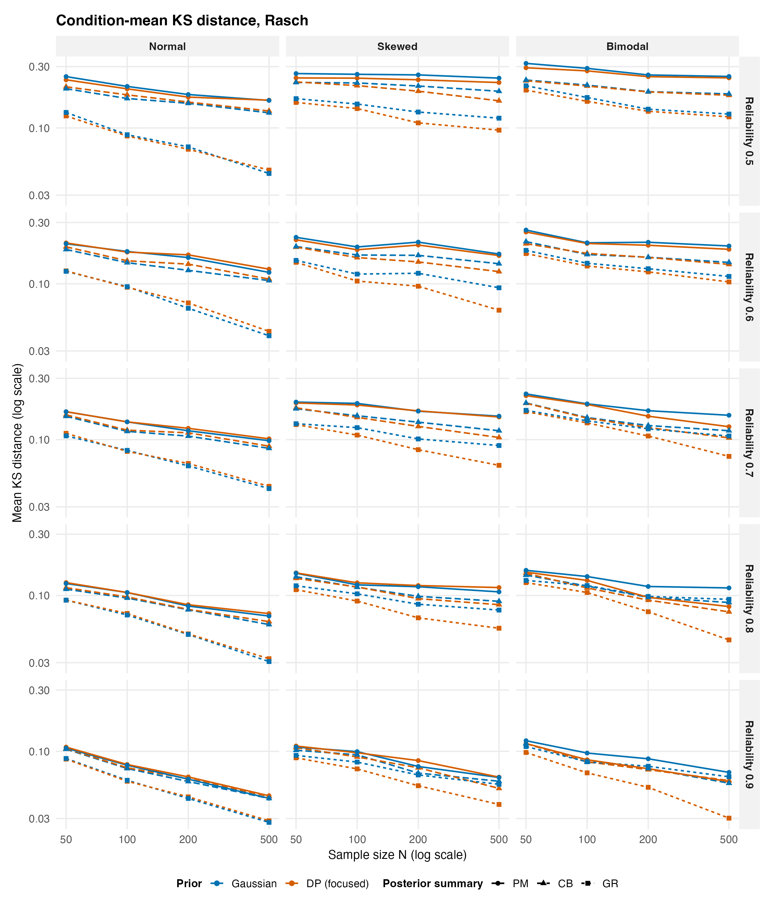
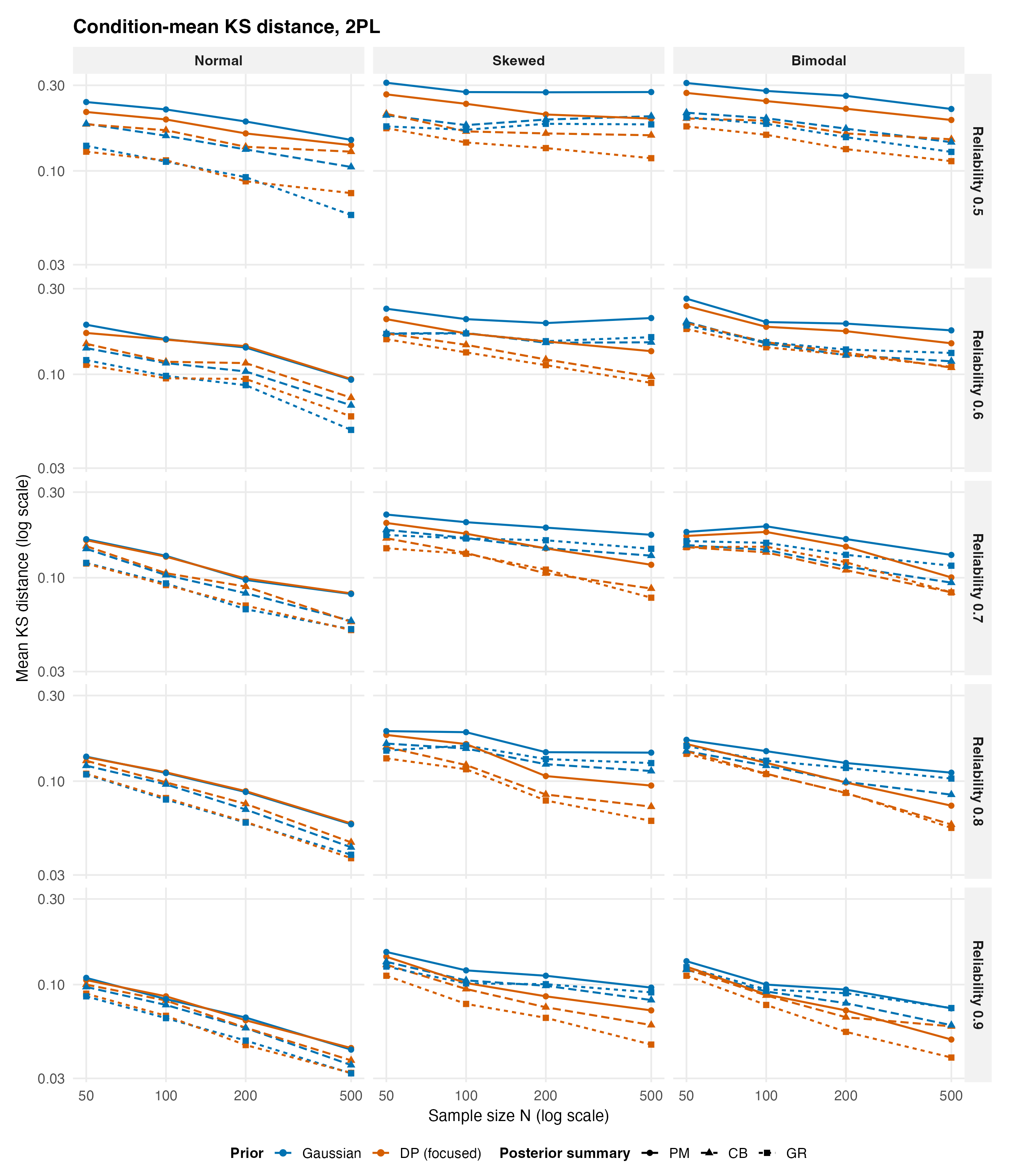
Three features of the raw scale matter downstream. Losses generally fall with N, with local non-monotonic points visible rather than suppressed. The three summaries usually separate the curves far more than the two priors do; this is the first appearance of a pattern that Chapter 9 quantifies. The broad Rasch ordering is not literally universal under the 2PL: the joint caption identifies its pointwise CB/GR and one high-tier exception. Finally, the two GR curves used by the primary contrast separate most visibly in informative non-normal regions, where the preregistered hypotheses expect the flexible prior to work.

8.2 The preregistered result

The primary contrast fixes the summary at GR on both sides and asks what the prior is worth. H1 states that the mean log KS ratio of DP (focused) + GR to Gaussian + GR is negative over the non-normal cells; H2 states that the ratio’s slope in log2(N) is negative, so the advantage grows with sample size. Both are supported at any conventional level. At the design’s center the H1 estimate is -0.221 (SE 0.013, 95% CI [-0.246, -0.195], Holm-adjusted p \(= 1.4 \times 10^{-28}\)), a loss ratio of .80; H2 estimates the per-doubling slope at -0.114 (95% CI [-0.123, -0.106]), so each doubling of N multiplies the ratio by about .89. Exact family tables are in Chapter 15.

Figure 8.2 lays the same contrast out cell by cell, with the locked evidence labels overlaid.

Figure 8.2: The flexible prior’s distribution-recovery advantage concentrates where reliability, sample size and non-normality meet. Each tile is the ratio of condition-mean KS distance for DP (focused) + GR against Gaussian + GR; blue marks ratios below 1 (the flexible prior recovers the latent distribution better), red above 1, printed values are the ratios. Outlined tiles carry a win or strong-win label under the locked evidence-map rule (bootstrap interval below 1 or 0.95); an x flags the cells whose interval sits entirely above 1. The normal columns are the negative control: ratios there hover near 1, no cell earns a win label, and in three cells the flexible prior’s small loss increase is itself resolved (interval above 1, largest ratio 1.32 at 2PL, reliability 0.5, N = 500). Ratios are equal-form-weighted means over 20 replications per cell; interval logic follows the preregistered rule with B = 10,000 hierarchical bootstrap replicates.

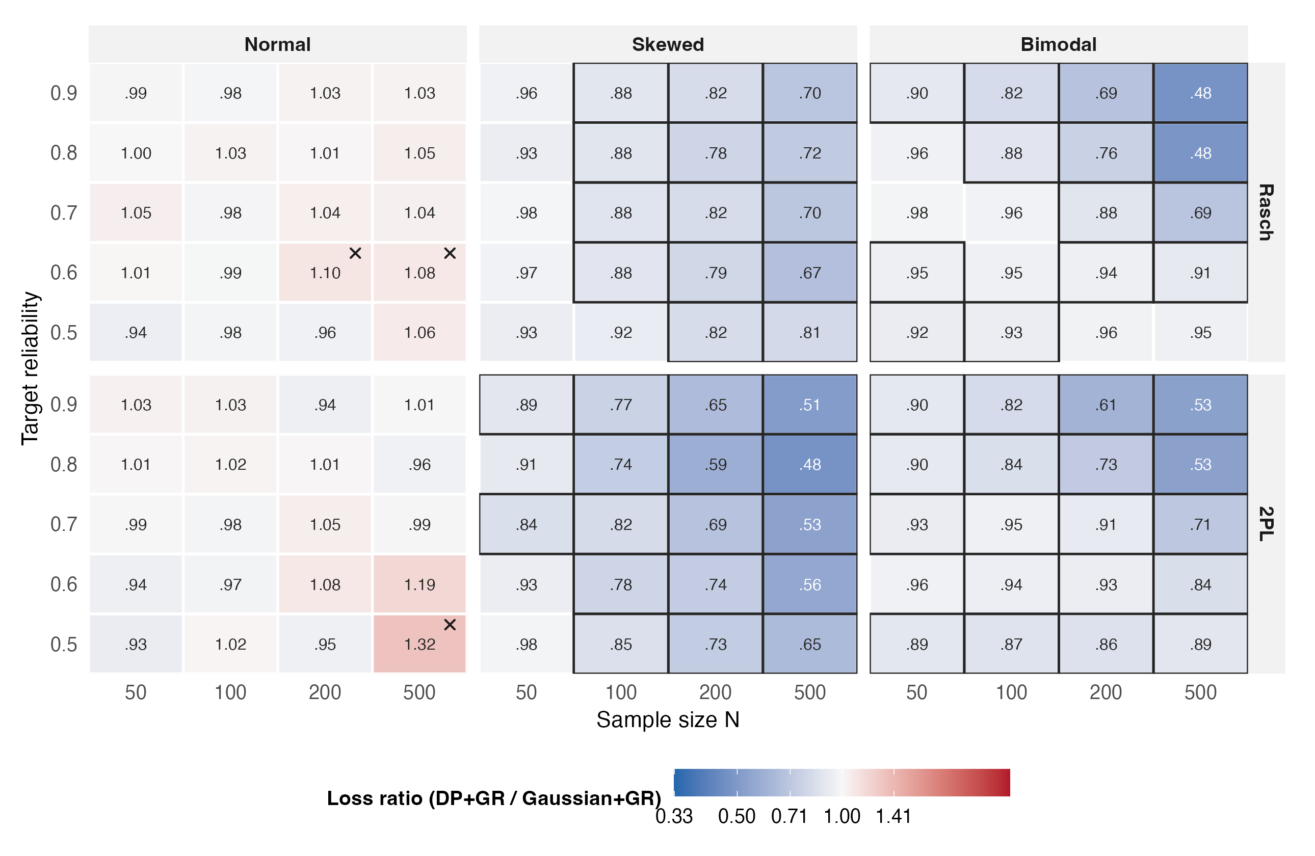
The geography is simple to state. Blue deepens toward the lower-right of each non-normal panel, reaching .48 where reliability 0.8 to 0.9 meets N of 500; the normal columns sit at parity apart from three cells in which the interval resolves the flexibility cost itself (the largest, 1.32, at 2PL, reliability 0.5, N = 500). The win labels outline the region where the bootstrap interval clears 1, which is the interior of the non-normal panels from N = 100 upward.

8.3 The advantage as a function of N, and the shape asymmetry

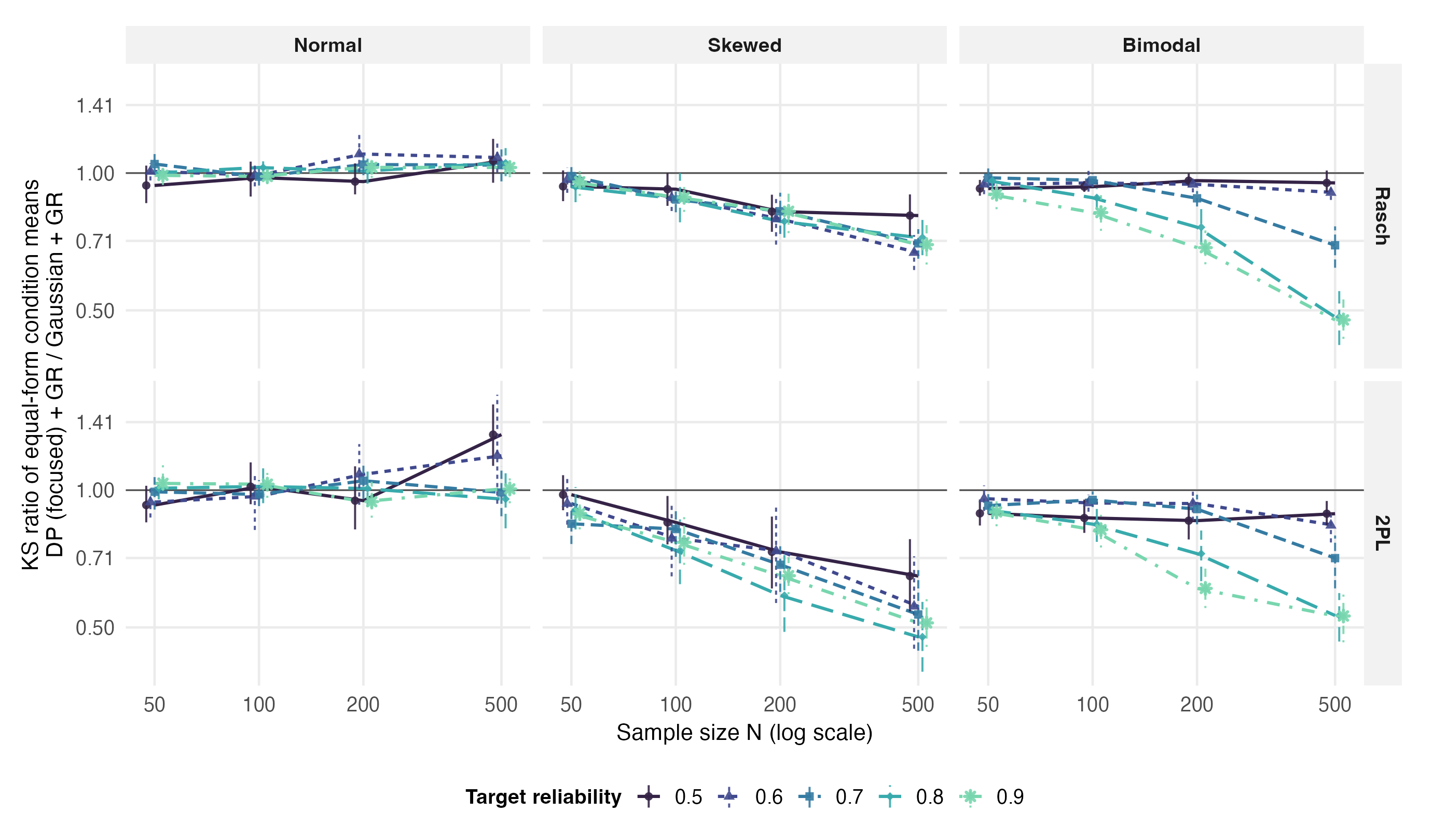
Figure 8.3: The flexible prior’s advantage generally grows with sample size; reliability separates the bimodal trajectories without eliminating low-tier gains. Each line traces rr_point, the ratio of equal-form condition-mean KS losses for DP (focused) + GR against Gaussian + GR, across sample sizes, one line per target reliability tier. Both axes are logarithmic, and the horizontal line at 1 marks parity. Vertical segments are 95% hierarchical-bootstrap intervals (B = 10,000) for that ratio of condition means; this is not the paired-geometric estimand. The normal controls mostly cluster around parity, with isolated departures. In the skewed columns the advantage grows with N at every tier. The bimodal lines fan more strongly: the 0.8 and 0.9 lines approach 0.5, but the 0.5 and 0.6 lines can also move materially below 1 as N grows. For example, the 2PL ratios are 0.857 at reliability 0.5 and N = 200 and 0.837 at reliability 0.6 and N = 500; the corresponding Rasch reliability-0.6, N = 500 ratio is 0.906. Low reliability attenuates the bimodal advantage in this grid; it does not impose parity for every N.

Figure 8.3 resolves H2’s single slope into its parts, and an asymmetry appears that the preregistered family did not anticipate. In the skewed columns the reliability lines fall together: even at reliability 0.5 the advantage grows steadily with N, reaching ratios near .65 under the 2PL at N = 500. In the bimodal columns the lines fan apart, but the lower tiers do not remain at parity. Under the 2PL, the ratio reaches 0.857 at reliability 0.5 and N = 200 (95% interval [0.780, 0.937]) and 0.837 at reliability 0.6 and N = 500 ([0.768, 0.902]); Rasch reaches 0.906 at reliability 0.6 and N = 500. Thus low information attenuates the bimodal advantage relative to the 0.8 and 0.9 lines, which dive toward .50, but does not eliminate it at every N. A reading consistent with the trajectories is that test information and N jointly determine how much population-shape signal the flexible prior can exploit; the crossed ladder does not identify either ingredient’s separate causal role.

8.4 What a replication looks like

Condition-level summaries say which combination is better; they do not show what better looks like. Figure 8.4 plots the estimate-set EDFs of one N = 500 replication in three informative cells against the replication’s true abilities, six estimate sets per row: two priors crossed with three summaries. These selected-replication displays are illustrative and exploratory; their caption places the selected primary ratios within the 20 sibling replications from each condition.

Figure 8.4: In these replications the summary governs the spread of the estimate set and the prior governs its shape. Each panel overlays one estimate-set EDF on the same replication’s true-ability EDF, for one N = 500 dataset per row; columns are three summaries applied to two fitted priors. Color and line type identify truth and prior. The low-reliability Rasch PM and CB estimates form score-associated bands while retaining visible within-band variation; both fitted PM series contain 500 distinct point estimates. That pattern is consistent with joint estimation of item and population parameters, rather than a score-only support rule. GR spreads estimates by estimated rank and restores a fuller range, while the prior affects recovered shape most clearly in the high-reliability rows. In-panel numbers are stored KS distances and reproduce frozen loss rows to within 1e-8. For the displayed rows, the selected DP-focused/Gaussian GR KS ratios are 0.44 (about the 50th empirical percentile; sibling range 0.33-0.71); 0.99 (about the 80th empirical percentile; sibling range 0.86-1.37); 0.60 (about the 80th empirical percentile; sibling range 0.33-0.85) among the 20 sibling replications in their respective conditions. Those empirical percentiles and ranges disclose selection sensitivity; they neither provide pointwise uncertainty for the displayed EDFs nor make these exploratory patterns representative or inferential.

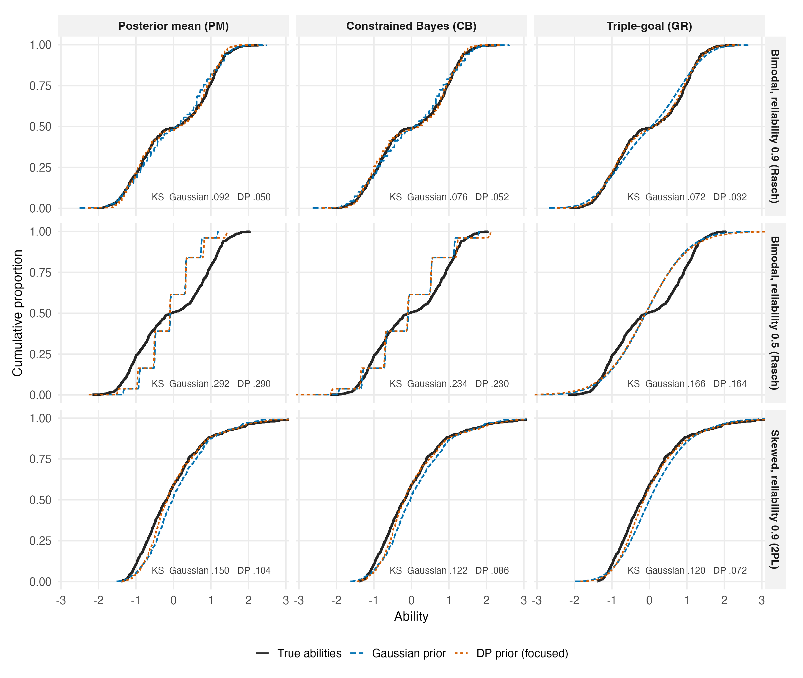
Two patterns organize an exploratory reading of the figure. First, at reliability 0.5 the eight-item Rasch form’s PM and CB estimates organize into visible score-associated bands while retaining within-band variation; both fitted PM series contain 500 distinct point estimates. This pattern is consistent with coarse response-score support combined with joint item and population estimation, but a selected replication cannot identify that mechanism on its own. GR spreads estimates by estimated rank and produces a fuller-range EDF in these panels. Second, the displayed GR curves have similar spread while their prior-specific shapes differ. In the top row (bimodal, reliability 0.9) the DP curve tracks the plateau in the true EDF that the Gaussian curve smooths away, and the stored KS values (0.032 against 0.072) are the vertical distances visible in the panel. In the middle row (reliability 0.5) the two priors are nearly indistinguishable, which is the fan of Figure 8.3 seen from inside a single dataset. These are descriptions of selected fits, not separate evidence that assigns the observed differences to one causal mechanism.

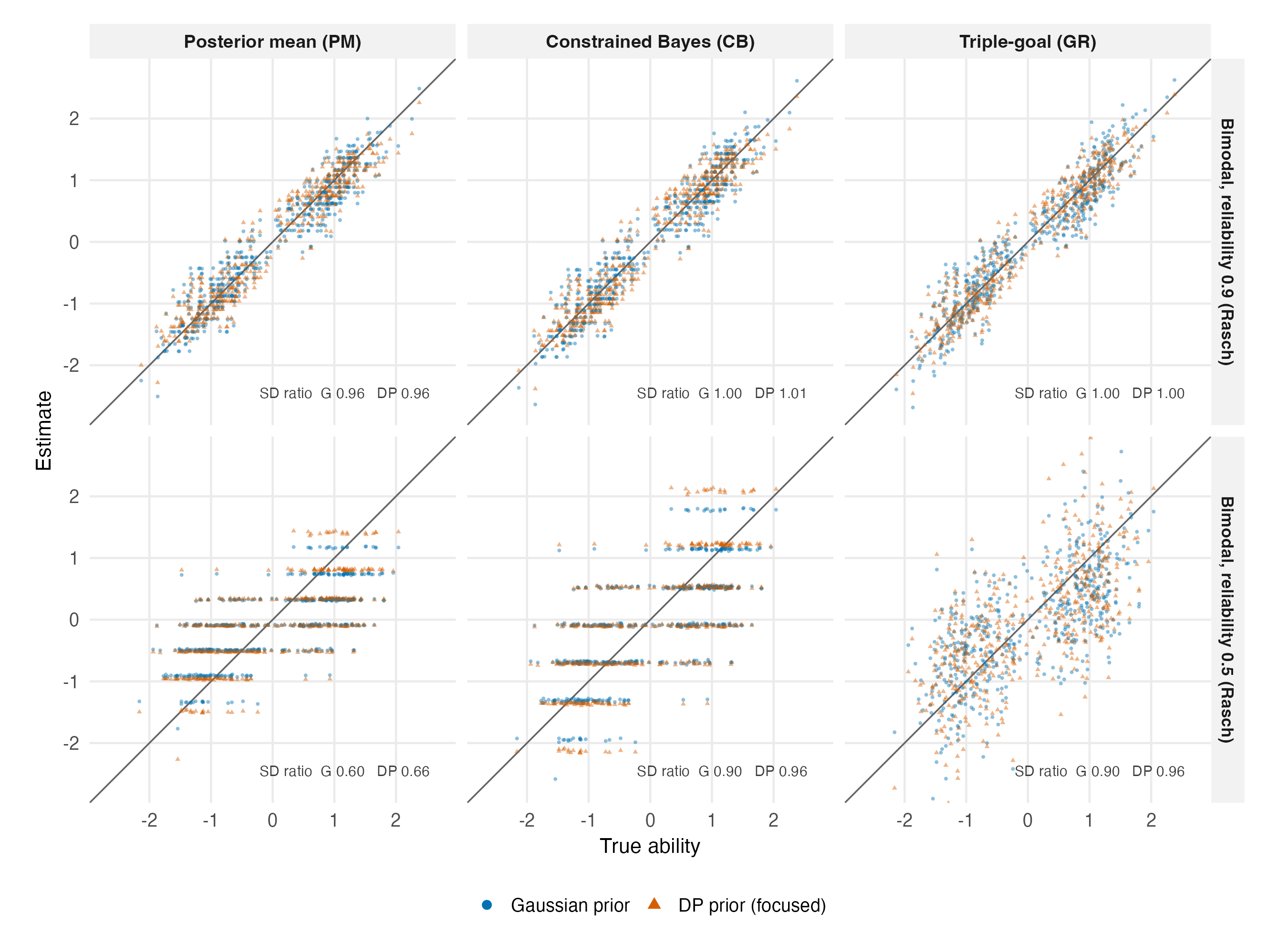
The same replications, plotted person by person, show the pattern from the individual side. In Figure 8.5 the estimate-versus-truth clouds tilt below the diagonal under PM, organize into score-associated horizontal bands with within-band variation at reliability 0.5, and show fuller spread under GR at both tiers. The remaining vertical scatter demonstrates that matching spread is not equivalent to recovering order; Chapter 13 provides separate condition-level descriptive evidence about rank loss.

Figure 8.5: In these replications the posterior mean compresses the estimate spread and GR restores it, while the ordering error within the cloud remains. Estimates are plotted against true abilities for one N = 500 bimodal replication at reliability 0.9 (top) and 0.5 (bottom), with color and marker shape distinguishing priors; the diagonal is perfect recovery. At low reliability, PM and CB form score-associated horizontal bands with visible within-band variation; the two fitted PM series each retain 500 distinct point estimates. This is consistent with joint item/population estimation rather than a score-only support rule. CB rescales the bands; GR spreads estimates by estimated rank but cannot repair ordering error. This is an exploratory pattern display, not a condition-average result. The selected high- and low-reliability DP-focused/Gaussian GR KS ratios are 0.44 (about the 50th empirical percentile; sibling range 0.33-0.71); 0.99 (about the 80th empirical percentile; sibling range 0.86-1.37) among 20 siblings per condition. The percentile/range check limits a simple cherry-picking concern but does not provide pointwise uncertainty for the displayed clouds.

8.5 Choosing within the DP family

The design carries two DP arms so that the elicitation choice is itself tested. The focused arm calibrates its concentration prior so that few clusters are expected a priori; the broad arm leaves the concentration diffuse. H5 states that focused beats broad on the primary response, and its primary estimate favors focused by about one percent: the mean log ratio is -0.01099 (95% CI [-0.017, -0.005], Holm-adjusted p \(= 0.000\)). Figure 8.6 shows how small that difference is in absolute terms: the two arms’ condition means sit on the identity line, and the evidence map labels 106 of 120 cells ties.

Figure 8.6: Descriptive H5 display: the two DP arms are close to interchangeable. Panel (a) plots each condition’s mean KS distance under the broad DP prior against the focused DP prior, GR summary; points sit on the identity line across all shapes and regimes. 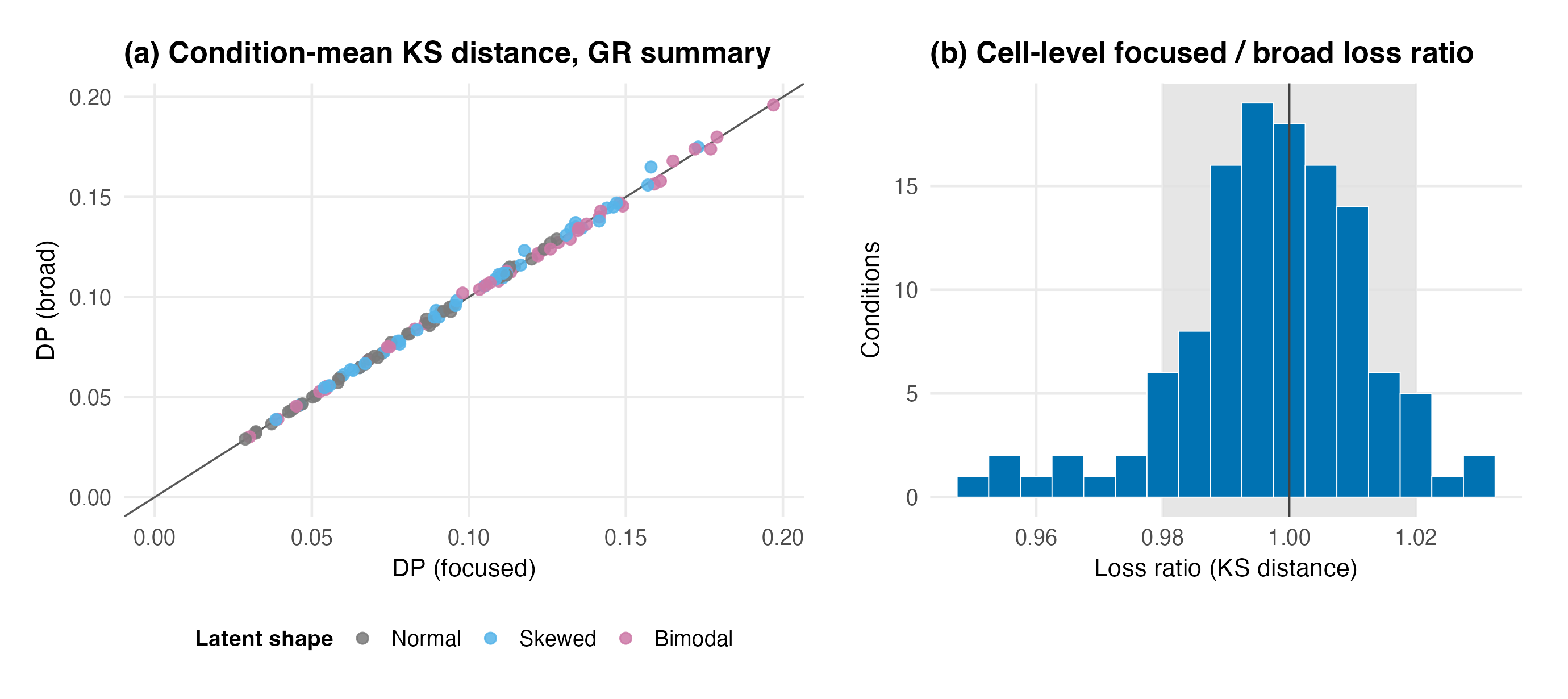Panel (b) shows the distribution over the 120 conditions of the paired geometric-style focused-to-broad ratio: the exponential of the equal-form mean of form-mean paired replicate log ratios (ratio_cells). It is not the evidence map’s rr_point, which is a ratio of equal-form condition means. The shaded band marks paired geometric-style ratios within 2 percent of parity. Separately, the registered primary H5 contrast puts the focused arm ahead by about 1 percent on average (log ratio -0.01099; loss ratio 0.989), and the rr_point evidence map labels 106 of 120 cells as ties. Under strict-pass-only filtering, the estimate attenuates to -0.00284 (two-sided 95% CI [-0.00610, 0.00042]); the registered directional one-sided Holm p-value is 0.0399. The display supports focused as a defensible default, not a practically large focused-over-broad advantage.

We read H5 as reassurance rather than as a forceful recommendation. In the strict-pass-only sensitivity, the focused advantage attenuates to -0.00284 with a two-sided 95% CI of [-0.00610, 0.00042]. The registered directional, one-sided Holm test remains just below 0.05 (\(p = 0.0399\)), but the two-sided interval includes zero. Thus the focused elicitation is a defensible default within the studied DP implementations, while a reasonably diffuse concentration prior appears to concede little on this response; the data do not support a practically strong claim that focused is superior. Full sensitivity results are in Section 14.5.

8.6 Reading the flags honestly

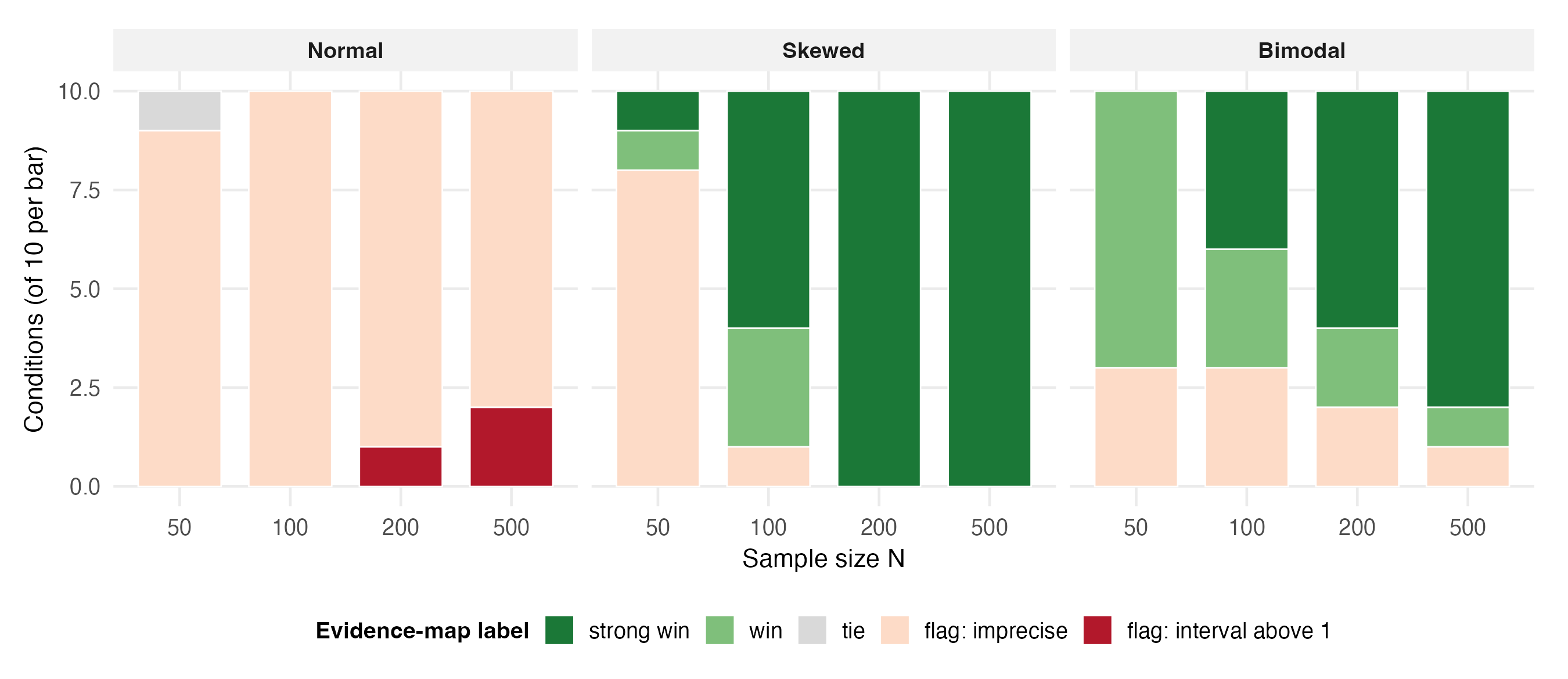
The evidence map labels 45 of 120 primary-contrast cells strong wins, 17 wins, 1 tie, and 57 flags. A flag is earned whenever the bootstrap interval neither clears 1 nor fits inside the tie band [0.95, 1.05], and it is tempting to read the flag count as evidence of widespread harm. It is not, and the decomposition matters. Of the 57 flags, 49 have intervals spanning 1 (the cell cannot distinguish a modest advantage from a modest cost), 5 have intervals entirely below 1 that merely fail the win rule’s point threshold, and 3, all in the normal columns, resolve an actual cost of flexibility. Figure 8.7 stacks the labels by sample size and shape. The flag count falls from 20 at N = 50 to 11 at N = 500, but this is not an interval-narrowing result: median log-interval width rises from 0.130 to 0.214. At the same time the median absolute log loss ratio rises from 0.058 to 0.303, so point estimates move farther from parity and more often clear the evidence rule (Section 14.4).

Figure 8.7: Most flags are imprecision, not harm, and they concentrate where information is scarcest. Locked evidence-map labels for the primary contrast, stacked over the ten conditions (two model families x five reliability tiers) at each sample size and shape. Wins and strong wins accumulate with N in the non-normal columns; the flag category splits into cells whose bootstrap interval simply fails to fit inside the tie band (imprecise, pale) and cells whose interval sits entirely above 1 (red). The flag label is a residual category, not a harm verdict: of its 57 cells, 49 have intervals spanning 1, 5 sit entirely below 1 while falling short of the win rule, and only 3, all normal-shape, resolve higher loss under flexibility. The individual-accuracy harm reported with the safety map lives on a different contrast (MSEL) and does not appear here.

8.7 What this chapter establishes

Under non-normal populations, replacing the Gaussian prior with a focused DP mixture while keeping the GR summary reduces distribution-recovery loss by about 20 percent at the design’s center, by 27 percent averaged over the preregistered opportunity region, and by half in the most informative corner; the advantage grows with N everywhere for skew and is steepest above reliability 0.7 for bimodality, with smaller but resolved gains in some 0.5 and 0.6 cells; the primary H5 estimate favors focused by about one percent, but that difference attenuates and has a two-sided interval spanning zero under the strict-pass sensitivity; and the flag half of the evidence map is dominated by small-N imprecision, with the only resolved costs being three normal-shape cells of at most 32 percent. What the chapter does not establish is equally definite: nothing here concerns individual-level accuracy, whose separate and less favorable arithmetic is the subject of Chapter 12.