9  The larger lever

The previous chapter treated the prior as the intervention and held the summary fixed. This chapter reverses the question. A practitioner who inherits the operational default, a Gaussian prior summarized by the posterior mean, has two alternatives available: model the ability distribution flexibly, or keep the model and change what is computed from the posterior. The two alternatives differ enormously in computational demand. The first multiplies the sampler budget and adds a truncation, an elicitation and a convergence surface to manage; the second is a few lines of post-processing on draws that already exist. The study’s design crosses the two completely, so it can say which alternative moves the loss more, where, and by how much. The comparisons in this chapter beyond the registered H7 contrast are exploratory in the preregistration’s sense: they were not part of the locked family, and no error rate is claimed for them.

9.1 Two levers, measured on the same scale

For every condition and loss family we compute two within-cell ranges over the nine condition-mean losses: how far the loss moves when the summary is swapped with the prior held fixed, and how far it moves when the prior is swapped with the summary held fixed. Figure 9.1 shows the distributions of the two ranges over the 120 conditions.

Figure 9.1: For four of the five goals, swapping the posterior summary moves the loss far more than swapping the prior. For every condition and loss family we compute two ranges over the nine condition-mean losses: the ratio of the worst to the best summary with the prior held fixed (averaged over priors), and the ratio of the worst to the best prior with the summary held fixed (averaged over summaries). Slabs show the distribution of these ranges over the 120 conditions; points give the median and the intervals the central 66% and 95%. On the distribution-recovery families the summary swap moves loss by a median factor of 1.45 (KS), 1.85 (quantile) and 2.08 (tail), with upper tails beyond 3, while the prior swap moves it by a median of 8 to 32 percent; on squared error the medians are 1.17 against 1.06. The rank family is the exception in both directions: neither lever moves it (medians 1.00 and 1.01; the axis is logarithmic). Within-cell descriptive factorial sums-of-squares shares attribute 79 to 82 percent of the nine-cell spread to the summary main effect for the KS and squared-error families; the residual interaction is not sampling error. 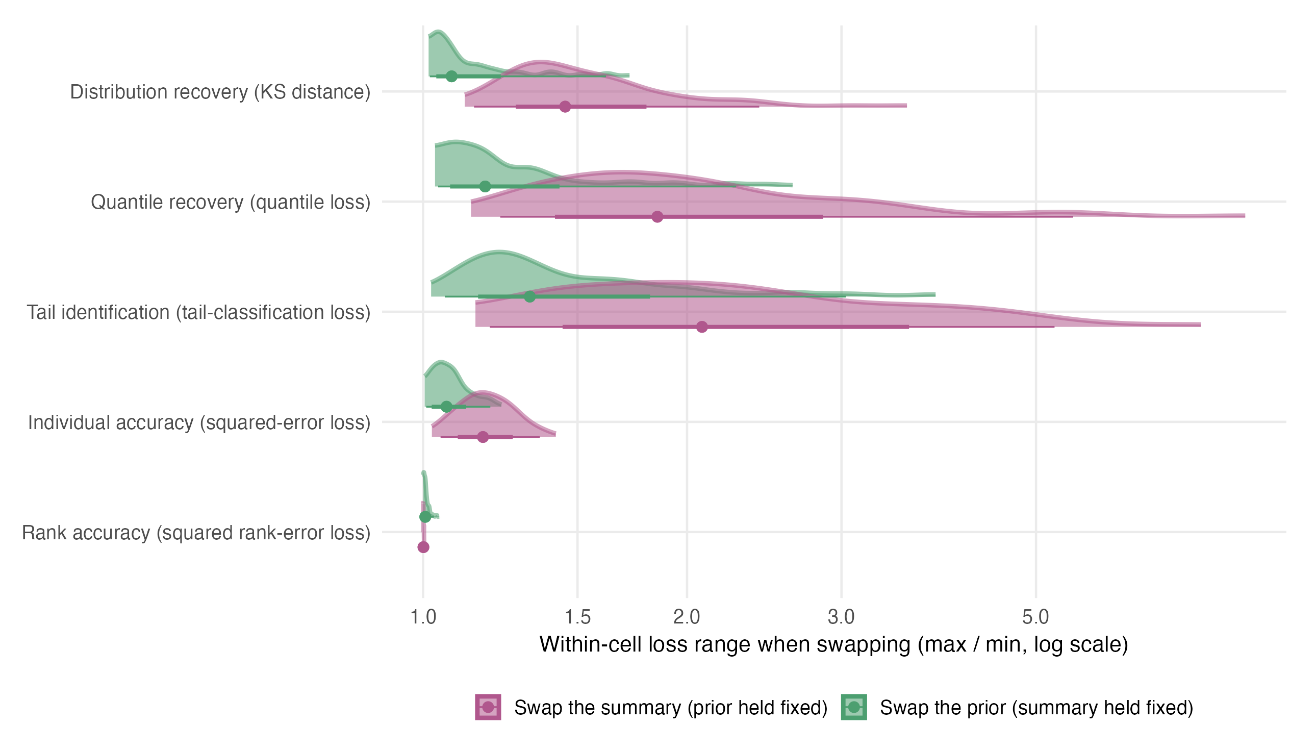The half-eye slabs use normalize = 'groups', which rescales each slab’s height within its group for viewing and does not encode group size or evidence weight.

Across the studied grid, the asymmetry is large and consistent. On the KS family the summary swap moves the condition-mean loss by a geometric-mean range factor of 1.52 against 1.13 for the prior swap; on the quantile and tail families the summary factors reach 2.01 and 2.24. A descriptive two-way factorial decomposition of the nine log means within each cell assigns 82% of their spread to the summary main effect on the KS family and 14% to the prior, with similar shares for squared error; its interaction residual is not sampling error. The rank family is the exception in both directions, and it is an exception of a special kind: neither lever moves it (Chapter 13). Being ranges over three levels, these figures measure the stakes of each choice, not an average effect; the stakes of the summary choice are simply several times higher almost everywhere.

9.2 What the summary is and is not given for free

A comparison of this kind invites an objection that we state before relying on it. The GR summary is constructed to reproduce an estimated distribution and an estimated ordering, and the distributional losses are computed on exactly those features; the posterior mean is constructed to minimize squared error, and the individual loss is exactly squared error. Each summary therefore enters its own goal with a built-in advantage, and neither “GR wins the KS comparison” nor “PM wins the squared-error comparison” is by itself informative.

Two things in the comparison are not settled by construction. The first is the size of the asymmetry. Averaged over priors, shapes, families and sample sizes, using PM where the goal is distributional costs 73 percent of KS loss at the two lowest ladder tiers and 31 percent at the two highest; using GR where the goal is individual accuracy costs 23 percent and 12 percent in the same bands. The mismatch penalties run in both directions, as construction implies, but they are roughly three times larger in one direction than the other, and both shrink as information rises. That ratio is a property of the design and the estimators, not of the definitions.

The second, and the reason the prior lever survives at all, is that GR matches an estimated distribution while the loss is measured against the realized one. Nothing in its construction guarantees that the distribution it reproduces is the right one: given a Gaussian prior and a bimodal population, GR faithfully reproduces a unimodal estimate. What GR removes is the ensemble compression that shrinkage imposes on the posterior mean; what remains after it is removed is the prior’s error about shape. That is why the two levers compound rather than substitute (Section 9.4), and why the flexible prior’s measured advantage in Chapter 8 is largest precisely in the cells where GR has already cleared the compression out of the way.

9.3 The registered dissociation

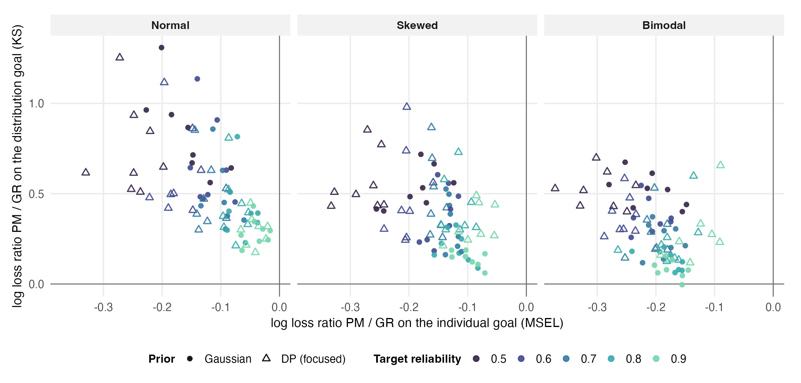
The lever comparison has a preregistered core. H7 states that the summary that minimizes loss depends on the goal: the PM-versus-GR gap should favor GR on the distributional loss and PM on squared error, and the difference of those two gaps should be positive. The estimate is +0.281 (SE 0.031, 95% CI [0.210, 0.351], Holm-adjusted p \(= 8.6 \times 10^{-6}\)). Figure 9.2 plots the two gaps against each other for every condition and both main priors. At the descriptive condition-mean point-estimate level, all 240 points sit in the quadrant where PM has lower squared error and GR lower KS loss. The plot carries no pointwise intervals, so this census is not 240 separate claims of resolved differences; H7’s registered mixed model supplies the pooled inferential statement.

Figure 9.2: At the condition-mean point-estimate level, the PM-versus-GR swap has opposite directions on the two goals in all 240 displayed condition-by-prior points. Each point’s horizontal position is the log condition-mean loss ratio of PM against GR on individual accuracy (negative means PM lower), and its vertical position is the same ratio on distribution recovery (positive means GR lower). All 240 point estimates occupy the upper-left quadrant. This census is descriptive and has no pointwise uncertainty intervals, so it is not 240 separate inferential claims. The registered H7 mixed-model contrast supplies the pooled test and estimates the mean dissociation at 0.28 log units (SE 0.03). Points are shaded by reliability; the narrowing vertical spread is an empirical pattern in this design.

9.4 Crossing the levers

The sharpest form of the question pits the two alternatives directly against each other: Gaussian + GR, a post-processing change, against DP (focused) + PM, a refitted flexible prior with the default summary. Figure 9.3 maps their ratio of equal-form condition-mean KS losses over the grid and reports the paired geometric-style ratio as a sensitivity.

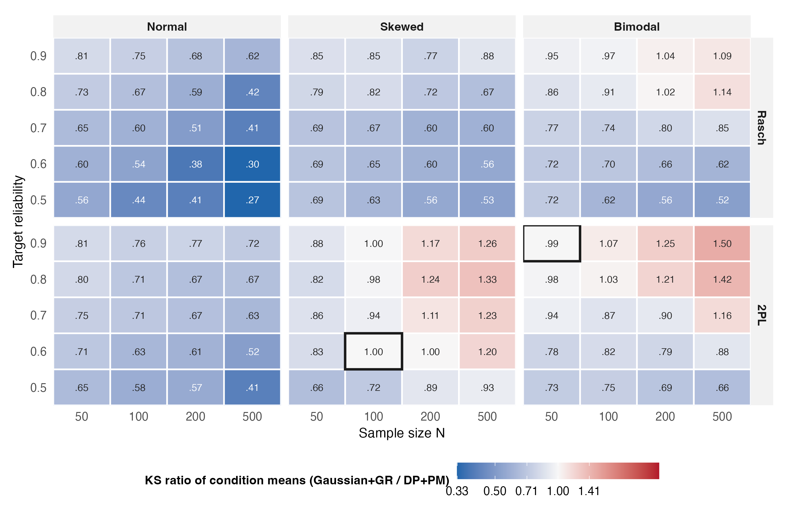
Figure 9.3: Gaussian + GR has lower loss than focused-DP + PM in 100 of 120 cells under either ratio convention, but the two exception rosters are not identical. Each tile is the cell-level KS ratio of equal-form condition means for Gaussian + GR against DP (focused) + PM, the rr_point aggregation used by the registered evidence maps (the crossed contrast itself is exploratory). Blue marks its 100 ratios below 1; 19 are above 1 and one equals 1. The paired geometric-style sensitivity, exp(mean(form-mean replicate log ratio)), likewise has 100 ratios below 1 and 20 above, but two cells switch classification; black outlines mark them. The paired exception roster is concentrated in non-normal higher-information cells but is not confined to N of 200 or 500: 2PL bimodal exceptions include N = 50 at reliability 0.9, N = 100 at 0.8 and 0.9, and N = 500 at 0.7. In the collapsed six-combination winner map, DP + GR wins 18 of these 20 paired exceptions and DP + CB wins two. Thus the exception region usually favors combining the flexible prior with GR, but not universally; the two ratio estimands remain distinct.

The two ratio conventions both put Gaussian + GR below DP (focused) + PM in 100 of 120 cells overall, but they do not classify exactly the same cells. In the displayed ratio of condition means, 19 cells are above 1 and one equals 1; in the paired-geometric sensitivity, all 20 exceptions are above 1. Two cells switch classification between the estimands. The paired exception roster is mostly higher-information and non-normal, but it is not confined to N of 200 or 500: the 2PL bimodal panel includes N = 50 at reliability 0.9, N = 100 at 0.8 and 0.9, and N = 500 at 0.7. Its largest ratio is 1.52. In the collapsed six-combination winner map, DP + GR is the winner in 18 of those 20 paired exceptions and DP + CB in two, so the flexible prior plus GR is usual there, not the only combination left standing. The winner map of Chapter 7 resolves the remaining competition cell by cell.

The comparison against the unimproved default completes the picture. The following aggregate percentages use the paired geometric-style cell ratios defined in Section 5.4 rather than ratios of condition means. Averaged over the non-normal cells, switching only the summary (Gaussian + GR against Gaussian + PM) reduces KS loss by 25 percent; switching only the prior (DP + PM against Gaussian + PM) reduces it by 12 percent, since with the posterior mean in place much of the flexible prior’s better representation of shape is shrunk away before it reaches the estimates; switching both reduces it by 41 percent, which exceeds what the two single swaps would compound to independently. The summary is the larger single lever, and the two levers reinforce rather than substitute: the GR summary is what lets a better prior show through in the estimates. This ordering is the clearest practical pattern in the studied grid.

9.5 The penalty matrix

Figure 9.4 condenses the summary question into an exploratory descriptive matrix. It reports geometric percentage penalties after finding the best summary separately at each exact reliability tier and then averaging log penalties into three display bands.

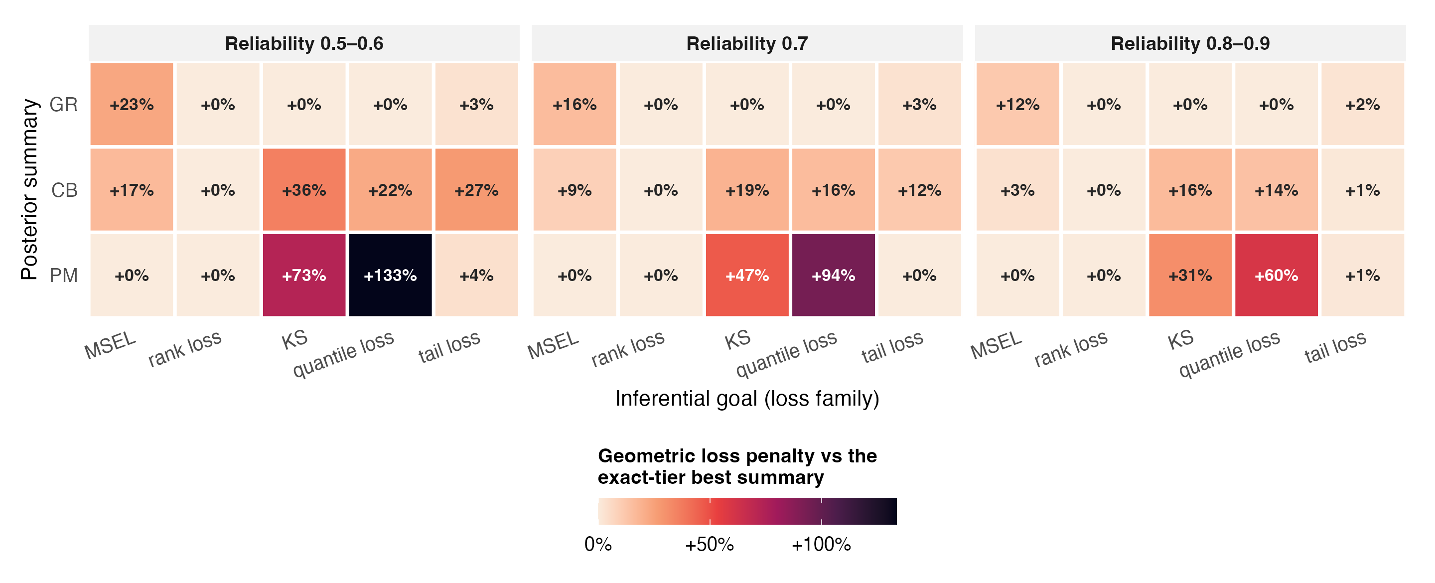
Figure 9.4: Summary penalties depend on the goal and, for tail loss, on the exact reliability tier. For each summary, goal and exact tier, the display first averages log raw equal-form condition-mean loss over the Gaussian and focused-DP arms, shapes, models and sample sizes. It then subtracts the exact-tier best log loss, averages those log penalties within the three displayed bands, and plots exp(mean log penalty) - 1. The cells are therefore geometric percentage penalties, not arithmetic average percentages. PM is exact-tier best for MSEL and GR for KS and quantile; the rank penalties are essentially zero. Tail loss has no single winner: from reliability 0.5 through 0.9 its exact-tier winners are GR, PM, PM, GR and CB. This exploratory matrix reads raw condition means, so the registered per-replicate comparator floor does not enter its estimand.

Reading along the rows: the posterior mean’s geometric penalty is 73 percent on KS and 133 percent on quantile loss in the low band, still 31 and 60 percent in the high band; CB sits between on those two goals. GR is exact-tier best for KS and quantile, while PM is best for MSEL; GR’s MSEL penalty falls from 23 percent in the low band to 12 percent in the high band. Rank penalties are essentially zero for every summary. Tail loss does not have one stable winner: the exact-tier sequence from reliability 0.5 through 0.9 is GR, PM, PM, GR and CB. The matrix is computed from raw equal-form condition means and never reads the registered per-replicate comparator floor, so the floor cannot explain its tail pattern.

9.6 What this chapter establishes

Across the studied distributional goals, the posterior summary is usually the larger lever by a factor of several, all 240 descriptive H7 condition-mean point estimates occupy the dissociation quadrant, and the registered mixed model supports the pooled contrast. The post-processing alternative has lower loss than the prior-only alternative in 100 of 120 cells under either ratio convention. The paired-geometric exceptions are mostly high-reliability, non-normal and 2PL, but include three 2PL bimodal cells at N below 200 and a reliability-0.7 cell at N = 500. Combining the flexible prior with GR produces the lowest observed loss in 18 of the 20 paired exceptions; CB does so in two. That region is the subject of the next chapter’s reliability analysis, and the individual-accuracy tradeoff accompanying these distributional gains is the subject of Chapter 12.