5 Estimands, losses, and contrasts – A Simulation Study of Dirichlet Process Mixture Priors and Goal-Specific Posterior Summaries in Bayesian IRT

5.1 Nine estimators

Table 5.1: The three prior arms. Item-parameter priors are common to all arms. Source: tables/T-arms.rds.

Arm	Prior on the ability distribution	Truncation M	Sampler budget
Gaussian	theta_i ~ N(mu, sigma^2), the default in operational IRT	-	8k/40k iterations (Rasch/2PL)
DP focused	DP mixture of normals; Gamma prior on the concentration calibrated so the prior expects few occupied clusters	50 (75 at N = 500)	12k/36k
DP broad	DP mixture of normals; deliberately diffuse concentration prior (sensitivity arm)	50-150 by N	12k/36k
Sources: sampler budgets are read from F$design (generated from data/design/sampler-budgets.csv); truncation schedules and prior descriptions are protocol constants from the frozen alpha-truncation manifest and production configuration.

Table 5.2: The three posterior summaries, computed from every fit. Source: tables/T-summaries.rds.

Summary	Decision problem it solves	What it preserves
PM (posterior mean)	minimize expected squared error for each individual ability	individual accuracy
CB (constrained Bayes)	minimize squared error subject to matching the mean and variance of the estimate set to the posterior expectations	first two moments of the ensemble
GR (triple-goal)	match the empirical distribution and ranks of the estimate set (Shen and Louis, 1998)	EDF and ranks of the ensemble

The crossing of Table 5.1 and Table 5.2 yields the nine combinations that populate the winner maps. The summary is computed from retained posterior draws, so its cost is post-processing only; the arm changes the fitted model and its budget.

5.2 Five losses

Table 5.3: The five theta loss families. Lower is better throughout; the item-parameter loss (beta, PM only) completes each fit’s loss record. Source: tables/T-losses.rds.

Family	Definition	Inferential goal	Confirmatory role
MSEL	mean squared error of individual ability estimates	individual scores	H4 safety
MSELR	mean squared error of percentile ranks (ties averaged)	ordering and selection	descriptive
KS	sup-distance between estimate and truth EDFs	distribution recovery	primary (H1-H3, H5, H6)
Quantile	weighted squared quantile gaps at deciles .10-.90	distribution recovery	sensitivity
Tail	weighted squared gaps in shares beyond cutoffs -2, -1.5, 1.5, 2	tail identification	descriptive; replicate-level registered ratios are floored
Source: preregistered loss definitions and roles, with replicate-level floor scope from Addendum 002 and H7 share-only floor scope from Addendum 003 amendment 001.

Three panels illustrating the largest empirical-distribution-function gap, horizontal gaps at five registered quantile probabilities, and outer-tail shares using lower tails at negative cutoffs and upper tails at positive cutoffs. — Figure 5.1: **What the three distributional losses measure.** All three compare the set of point estimates (blue; here the Gaussian-prior posterior means from one N = 500 bimodal replication at reliability 0.5, where shrinkage is severe) with the same replication’s true abilities (black). The KS distance (a) is the largest vertical gap between the two empirical distribution functions; the quantile loss (b) is a weighted sum of squared horizontal gaps at the five registered probabilities (0.10, 0.25, 0.50, 0.75 and 0.90). The tail-classification loss (c) uses the lower-tail event X <= c at negative cutoffs and the upper-tail event X >= c at positive cutoffs, exactly as in the production loss. Shrinkage nearly empties those outer tails in this example. The three losses respond differently: an estimate set can match the median while missing each registered outer-tail share.

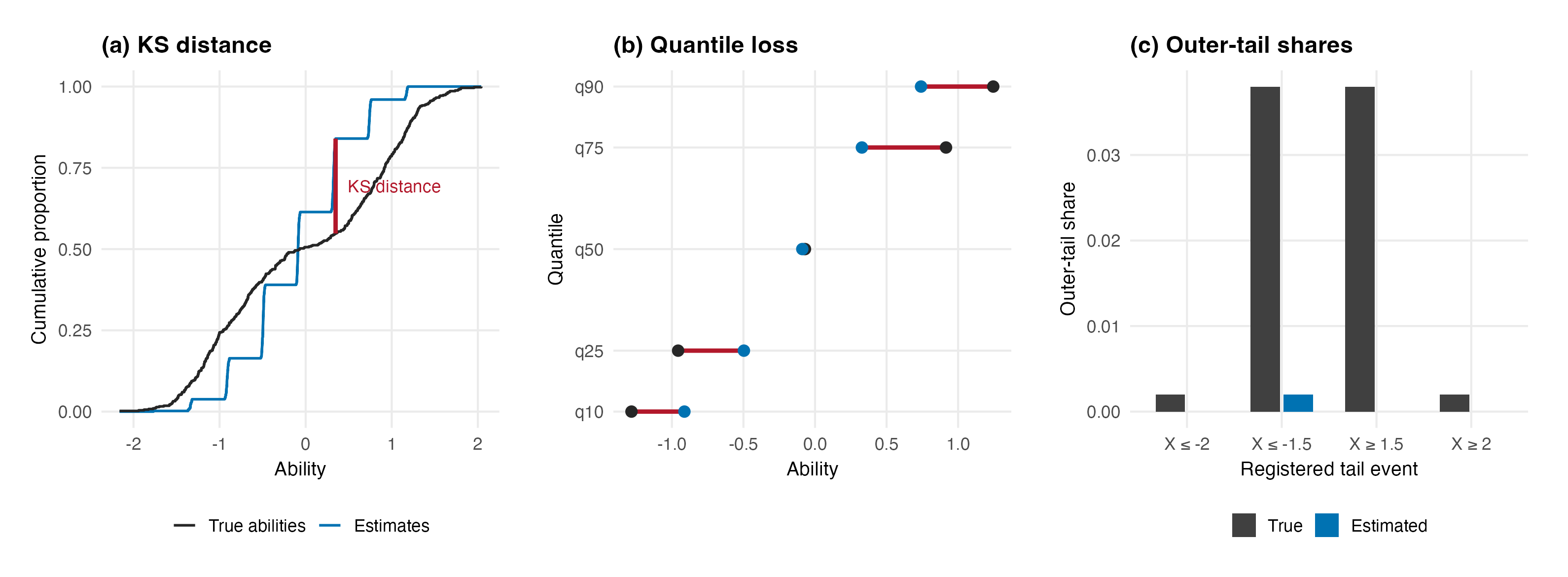
Every loss compares an estimate set with the same replication’s realized true abilities, not with the population’s analytic form; the estimand is recovery of this sample’s ensemble, which is what an operational report is about. Figure 5.1 draws the three distributional losses on one low-reliability exemplar, where their differences are visible. The KS distance is the primary distributional loss by preregistration; the quantile loss squares and weights gaps at the five registered probabilities 0.10, 0.25, 0.50, 0.75 and 0.90, so it amplifies the same discrepancies. The tail loss compares lower-tail shares at negative cutoffs and upper-tail shares at positive cutoffs and is the one family whose comparator can be exactly zero, the origin of the floor discussed in Section 13.3. Squared rank-error uses percentile-scaled ranks with ties averaged. The individual loss (MSEL) is squared error in the reporting metric.

5.3 One scale for all arms

Losses are computed on a common reporting scale, the standardized scale of the generating population. In this simulation, the known generating item difficulties and scaled discriminations stored with each frozen dataset define the map from the constrained-item fit scale back to that DGP scale before losses are computed. This truth-based alignment is available because this is a simulation; it is not an identification procedure available in an operational analysis with unknown generating parameters. Without the explicit map, arm comparisons would mix scale conventions with substance. The mapping was repaired and re-verified after an external review found the earlier convention leaking across a boundary (Addendum 005; the incident and its verification are part of Appendix D), and every loss row carries the scale identifier and map hash it was computed under.

5.4 From replicate to condition

Two cell-level ratio estimands appear in the book, and the nonlinear aggregation means they are not interchangeable. For the registered evidence maps, losses are averaged first. If $L_{A,cfr}$ is the loss for pipeline A in condition $c$, form $f$, and Monte Carlo replicate $r$, define the equal-form condition mean

\[ \bar L_{A,c}=\frac{1}{F}\sum_f\left(\frac{1}{R_f}\sum_r L_{A,cfr}\right), \qquad \mathrm{RR}^{\mathrm{mean}}_c=\frac{\bar L_{A,c}}{\bar L_{B,c}}. \]

The frozen evidence column rr_point is $\mathrm{RR}^{\mathrm{mean}}_c$. Its hierarchical bootstrap resamples forms and then paired replicates within form ($B = 10,000$). Registered cell labels and safety boundaries are attached to this ratio of equal-form condition means.

Some exploratory displays instead use the paired geometric-style cell ratio in ratio_cells:

\[ \mathrm{RR}^{\mathrm{paired}}_c =\exp\!\left[\frac{1}{F}\sum_f\left\{\frac{1}{R_f}\sum_r \log\left(\frac{L_{A,cfr}}{L_{B,cfr}}\right)\right\}\right]. \]

This second quantity preserves dataset pairing before aggregation. In general, $\mathrm{RR}^{\mathrm{mean}}_c\ne\mathrm{RR}^{\mathrm{paired}}_c$; equal form weighting does not remove the distinction. Each ratio-using figure identifies which quantity it displays. Confirmatory hypotheses operate on the registered replicate-level log-ratio rows and pool them in mixed models with a form-family random intercept (Section 6.4); their coefficients are therefore not cell-level ratios of condition means either.

5.5 Six contrasts and the label rule

Six contrasts were registered: the primary distribution-recovery contrast (DP focused + GR against Gaussian + GR on KS), its broad-arm companion, the within-DP comparison, the MSEL safety contrast on the same combination pair, the CB-against-PM summary contrast, and the normal-cell control. Each cell of each contrast receives a locked evidence label: win if the bootstrap interval lies below 1 (strong win if below 0.95), tie if the interval sits inside [0.95, 1.05], and flag otherwise. The flag category is a residual, not a verdict; Section 8.6 decomposes it. The safety contrast additionally carries the 1.05 and 1.10 boundaries whose block label is the claim gate’s trigger (Section 6.5). The registered point ratios and evidence labels use rr_point, the ratio of condition means defined above. Exploratory displays that use ratio_cells name the paired geometric-style estimand explicitly; neither is described as a substitute for the other.