2 The two levers
A Bayesian item response analysis ends with a joint posterior over abilities. Everything a report contains, scores, orderings, shares below a cutoff, is a functional of that posterior, and the analyst controls two separable choices on the way to it: the prior placed on the ability distribution, and the summary that turns each person’s posterior into a reported number. This chapter develops the two choices far enough that the results can be read with their mechanics in view. Formal statements and derivations are collected in Appendix C; the theory volume of this project treats them fully.
2.1 Shrinkage, and what it does to an ensemble
Write \(\theta_i\) for person \(i\)’s ability and \(G\) for the population distribution the study wants recovered. Under the hierarchical model the posterior mean \(\hat\theta_i^{\mathrm{PM}} = E(\theta_i \mid \mathbf{y})\) minimizes expected squared error for each person, and it does so by shrinking: each estimate is a compromise between the person’s data and the prior, weighted by their precisions. Shrinkage is not a defect; it is the mechanism by which the posterior mean earns its optimality. The defect appears only when the ensemble of shrunken estimates is treated as an estimate of \(G\). Averaging pulls every estimate toward the center, so the collection \(\{\hat\theta_i^{\mathrm{PM}}\}\) is systematically narrower than \(G\), and any functional of \(G\) that depends on spread or shape, a variance, a tail share, a percentile cutoff, inherits the compression. The size of the compression is governed by measurement precision, a fact quantified in Chapter 3 and approximated by a particularly simple reference calculation: under a normal–normal working model with constant measurement-error variance, the posterior-mean ensemble’s standard deviation is \(\sqrt{\rho}\) times the latent standard deviation. The general law-of-total-variance result is underdispersion; the \(\sqrt{\rho}\) factor is not an exact identity for the nonlinear, heteroskedastic IRT likelihood or for a DPM posterior.
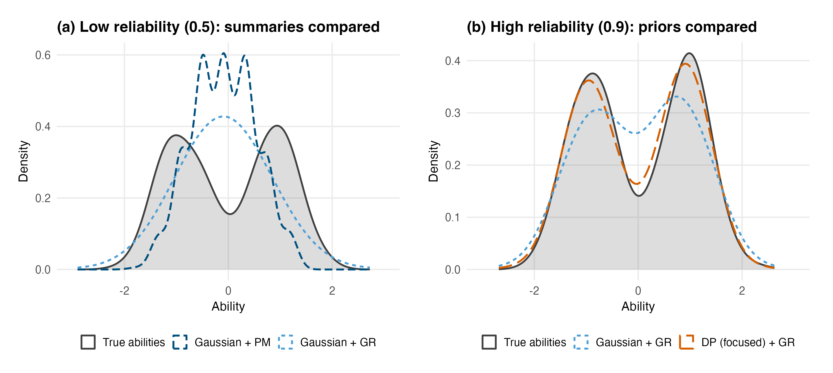
Figure 2.1 shows the phenomenon and both of the book’s levers acting on it in two selected bimodal replications from the study. The display is an exploratory mechanism illustration; its caption reports where the selected loss ratios fall among their sibling replications.
2.2 Summaries as answers to stated problems
The repair for underdispersion is not to abandon the posterior but to ask it a different question. Each summary in the study is tied to a distinct decision problem, and the study’s estimand map (Figure 2.2) organizes them by the question they answer. PM is the exact personwise squared-error action; the production CB and GR calculations are the finite-sample or finite-MCMC implementations described below and in Appendix C.
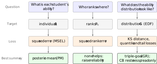
The posterior mean (PM) answers the individual question. The general constrained-Bayes (CB) action minimizes squared error subject to matching the joint posterior’s target ensemble mean and variance (Ghosh, 1992). The production implementation uses the posterior-independence specialization based on marginal variances rather than the full cross-person posterior covariance. Both forms are positive affine rescalings of the PM set, so they preserve PM ordering and standardized shape while changing spread; only the joint form exactly enforces the general posterior constraint. The triple-goal estimator (GR) of Shen & Louis (1998) goes further: it estimates ranks and the ensemble distribution, then assigns the corresponding estimated distribution quantile to each person. In this study, expected ranks and the pooled posterior EDF are approximated from retained MCMC draws, with type-8 interpolation used for the final quantiles. The resulting GR set has the estimated distribution’s shape and the estimated ranks’ order; its individual estimates can have higher squared error while improving ensemble recovery, a tradeoff this study measures (Section 12.3). All three summaries are computed from the same fitted posterior, so in the study’s design the summary is a within-fit factor: nothing about the model, the data or the sampler changes between them.
2.3 The prior lever: Dirichlet process mixtures
The second lever replaces the normality assumption on \(G\) itself. The study’s flexible arms place a Dirichlet process mixture (DPM) prior on the ability distribution: a DP prior (Ferguson, 1973) draws a random discrete measure, and a normal kernel at each atom smooths it into a density. Figure 2.3 walks the construction.
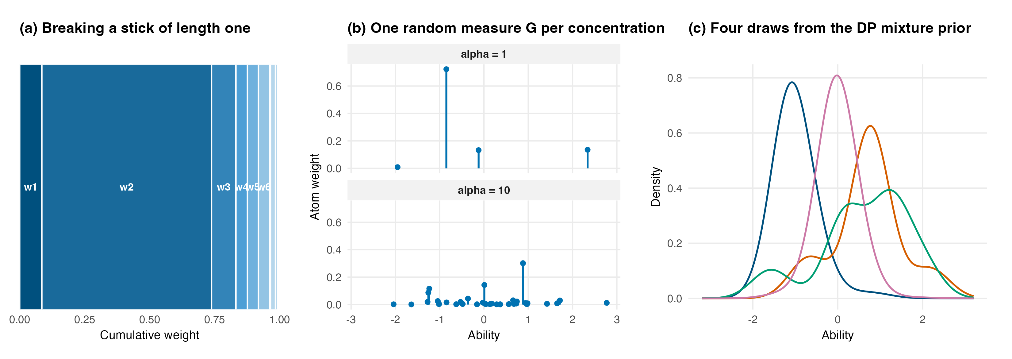
Two properties matter for reading the results. First, a normal-kernel DPM has enough support to represent densities close to normal, and a normal base-and-kernel construction can center its prior mean density on a normal shape. That support and centering do not make a DPM fit identical to the parametric Gaussian analysis: the parameter spaces, prior weights and posterior averaging remain different even when one cluster dominates. Whether the flexible model changes loss appreciably under a normal population is therefore an empirical question, which the study’s negative control addresses (Section 7.1). Second, the concentration parameter \(\alpha\) governs how readily the prior supports additional occupied clusters (Antoniak, 1974; Escobar & West, 1995), which makes its own prior a genuine modeling decision. The study fits two versions: a focused arm, whose Gamma prior on \(\alpha\) is calibrated by a numerical exact-moment procedure (Lee, 2026) so that the implied number of occupied clusters concentrates on small values, and a broad arm calibrated to a higher and more diffuse cluster-count target, so that the elicitation’s value is itself measured (H5; Section 8.5). The calibration machinery is summarized in Appendix C and treated in full in the theory volume; sampling uses the truncated stick-breaking representation with truncation levels recorded per fit (Section 14.2).
2.4 Why the levers must be studied jointly
Each lever has a literature; their pairing is less studied in IRT, and the results chapters show why the pairing is where the action is. The flexible prior changes what the posterior knows about shape; the summary changes whether that knowledge reaches the reported numbers. A DPM prior under PM summarization has its better shape estimate shrunk away before reporting (Section 9.4 shows this arithmetic cell by cell); a GR summary under a Gaussian prior faithfully reproduces a shape estimate that cannot bend away from normality. Only the combination among those studied lets both forms of flexibility reach the report, and only when the data carry such information. In this design, the prior controls the modeled range of population shapes, the summary controls how that posterior information enters the reported estimate set, and the measurement controls how strongly the data distinguish those shapes. The measurement component is the subject of the next chapter.