13  Ranks, quantiles, and tails

Three loss families remain. In this grid, the rank family varies overwhelmingly along the reliability axis and only slightly across the plotted estimators; the quantile and tail families largely repeat the KS story but each adds one caution worth recording. None of the three carries confirmatory weight (the quantile family was registered as a sensitivity companion and the tail family is descriptive), so this chapter is deliberately brief and plainly labeled: what follows is description with Monte Carlo error, not hypothesis testing.

13.1 Ranks: a dominant reliability gradient

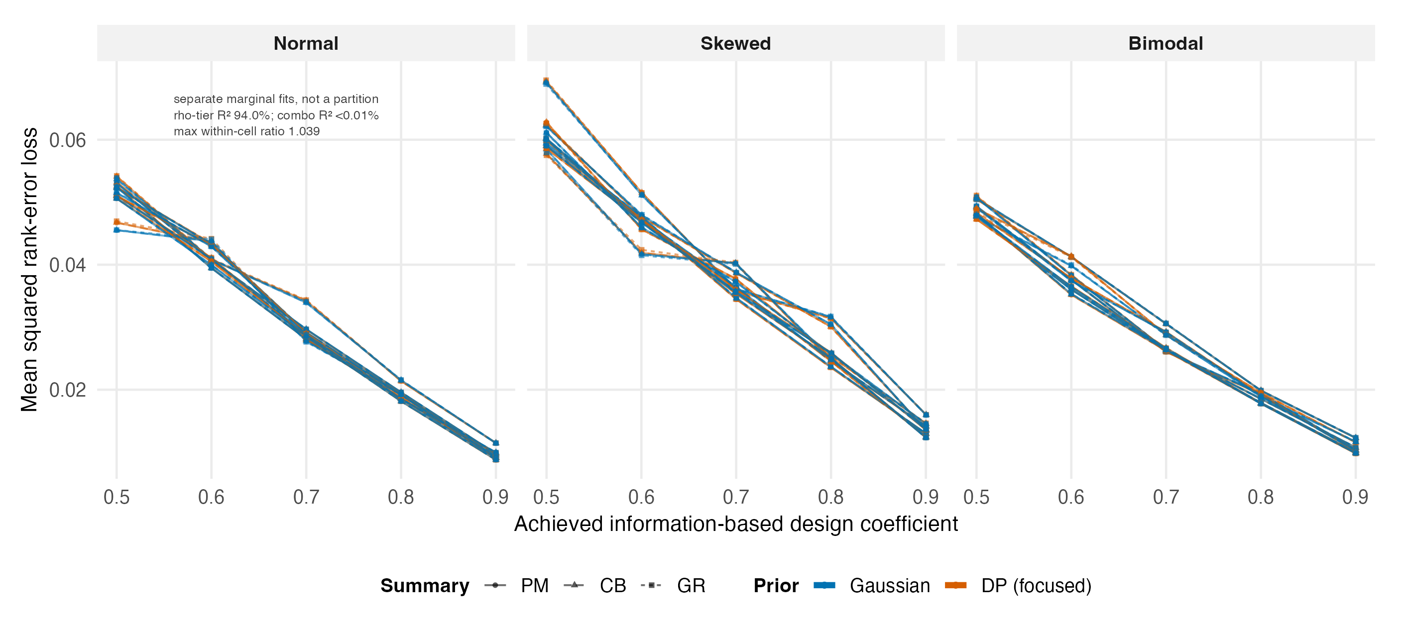
Figure 13.1: Rank loss varies chiefly with reliability in this descriptive grid. Condition-mean squared rank-error loss is plotted against the achieved information-based design coefficient. Each of the 48 lines per panel represents one of six prior-summary combinations within one model family and sample size; prior is encoded by color and summary by point shape and line type. Separate marginal regressions on log condition means give R² = 94.0 percent for reliability tier and less than 0.01 percent for combination, but those R² values are neither an additive variance partition nor an equivalence test. Across the six displayed combinations, the largest within-condition max/min loss ratio is 1.039. The overlap is therefore strong in this grid, without establishing that estimator choice has exactly zero effect outside it.

Figure 13.1 plots the condition-mean squared rank-error loss against achieved reliability, with one line for every combination of prior, summary, model family and sample size; 48 lines cross each panel and overlap closely. Two separate marginal regressions on the log condition means give \(R^2=0.940\) for reliability tier and \(R^2=0.00000022\) for combination. These values are not additive components of a variance partition and do not constitute an equivalence test. A more direct scale check reaches the same bounded descriptive conclusion: across the six plotted combinations, the largest within-condition max/min loss ratio is 1.039.

Rank loss is invariant to transformations that preserve the ordering, so PM, CB, and GR can separate only when they reorder people. In the methods and grid studied here, those differences are small relative to the information gradient. Programs focused on ordering should therefore consider test information first, while treating the near-overlap of these particular estimators as descriptive evidence rather than proof that no estimator could matter.

13.2 Quantiles: the KS story, amplified

Figure 13.2: The quantile family broadly echoes the KS geography, but its normal controls are not uniformly near parity. Tiles are ratios of equal-form condition-mean weighted squared quantile loss at the nine deciles from .10 through .90 for DP (focused) + GR against Gaussian + GR. They are ratios of condition means, not paired-geometric ratios, and are shown descriptively without interval labels. Blue deepens toward ratios near 0.25 in the high-information non-normal corner. Across the 40 normal cells the ratios instead range from 0.840 to 2.221, with four outside [0.9, 1.1]; thin black outlines identify those four cells. Because this loss squares quantile gaps, ratios can amplify small absolute discrepancies, especially when the Gaussian denominator is small. The map is therefore a descriptive sensitivity companion, not an uncertainty-qualified copy of the KS evidence map.

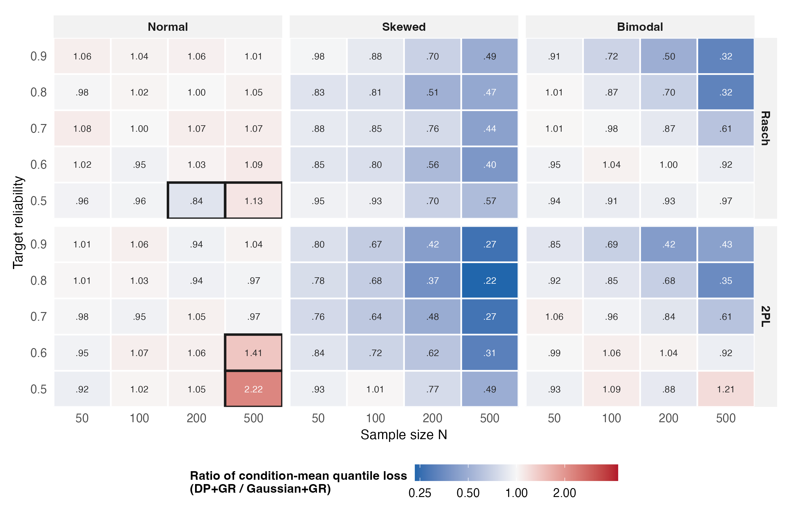
The quantile family orders the combinations the same way the KS family does, with GR first (96 of 120 winner cells) and the flexible prior’s territory in the same corner, but on a squared scale that often enlarges the log amplitudes: ratios reach .25 where the KS map shows about .50. The normal controls are an important departure from a simple copy of the KS map. Their 40 descriptive ratios range from 0.840 to 2.221, and four lie outside [0.9, 1.1], including 2PL, N = 500 cells at reliability 0.5 (2.2207) and 0.6 (1.4148). These are ratios of small squared-error denominators and carry no interval labels, so a reader should not treat their amplitude as uncertainty-qualified evidence. We therefore quote KS numbers in prose and use Figure 13.2 as a descriptive sensitivity companion.

13.3 Tails: a family governed by its floor

Figure 13.3: The registered replicate-level floor binds more as N grows; the raw condition-mean map in panel (a) is not floor-adjusted. Panel (a) maps the ratio of raw condition-mean tail-classification loss (cutoffs at -2, -1.5, 1.5, 2) for DP (focused) + GR against Gaussian + GR as a descriptive companion. Panel (b) shows the incidence of the separate registered replicate-level guard: its floor, a fixed share of each cell’s mean comparator loss, binds for 60 percent of comparator values at N = 50 and 85 percent at N = 500. Addendum 002 was logged after P-2 but before P-3 and production. It made that registered floor symmetric in the two operands and floored rather than dropped exactly-zero losses; it expressly does not apply to the raw condition-mean ratios in panel (a). Neither panel supports a confirmatory tail claim.

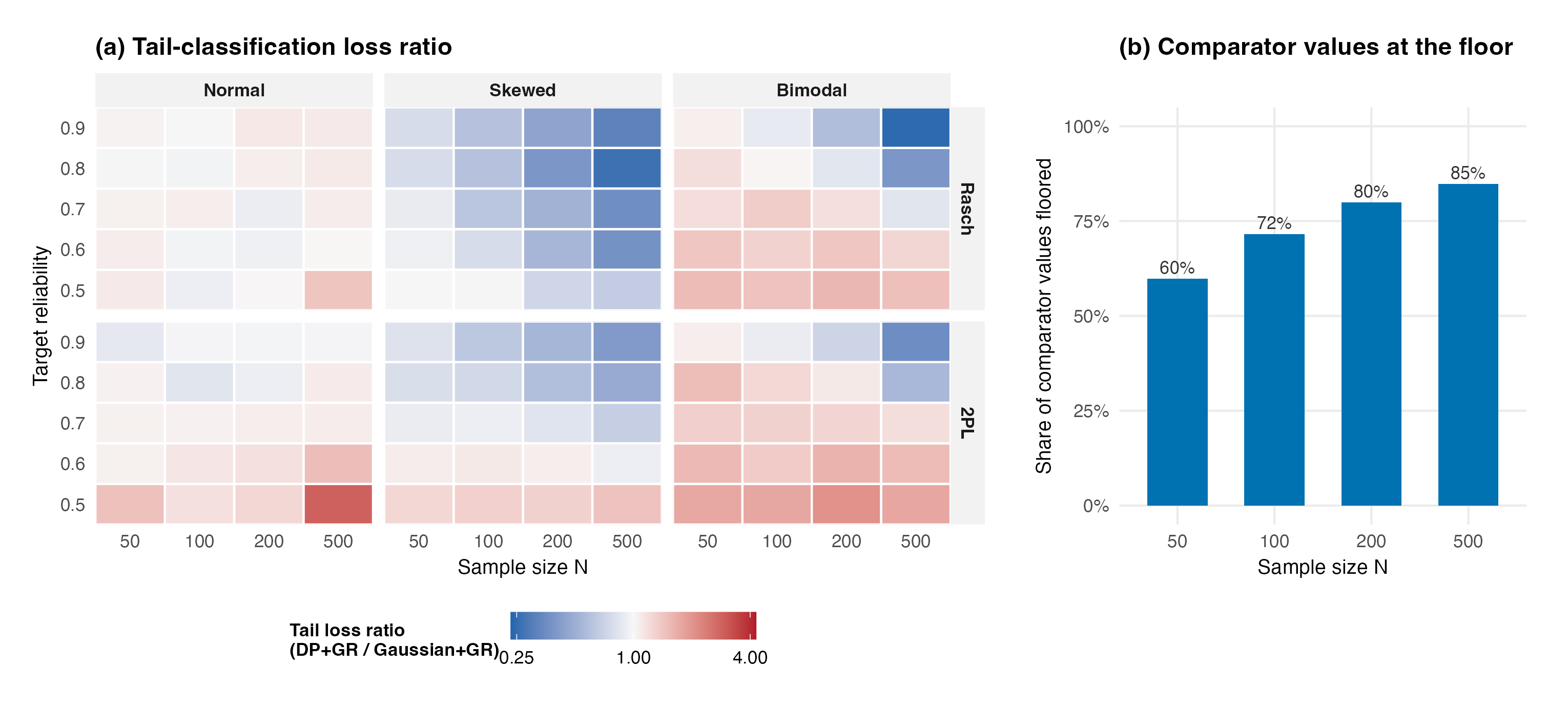
The tail-classification family was built to ask a screening question, what share of a population sits beyond fixed cutoffs, and it is the one family whose measurement apparatus intrudes on its answers. Either loss in a replicate-level ratio can be exactly zero, because an estimate set can match all four tail shares of a replication perfectly. The locked plan therefore sets a floor at a fixed share of the cell’s mean comparator loss. Addendum 002, logged after P-2 but before P-3 and production, fixed a defect in how that floor was being applied: the implementation floored the comparator only, which caps evidence against the flexible arm while leaving evidence in its favor unbounded, and dropped exactly-zero replicates rather than flooring them. The registered rule is symmetric in the two operands, with the floor’s scale still taken from the reference arm.

Its scope matters. Addendum 002 governs registered replicate-level log ratios. It does not govern the equal-form condition-mean ratios used descriptively in panel (a), which are computed from raw condition means and receive no floor. Panel (b) shows the incidence of the registered guard: the floor binds for 60 percent of comparator values at N = 50 and 85 percent at N = 500, because tail losses themselves fall toward zero as estimates sharpen while the floor, being a share of a cell mean, falls more slowly. The floor binds more, not less, as information grows, the opposite of what the concern registered before the wave anticipated. Panel (a) shows the same broad geography as the other distributional families (blue toward the informative non-normal corner, red in the bimodal low-reliability block), but its raw condition-mean ratios must not be attributed to the floor. We decline to treat either view as confirmatory evidence or to quote the ratios as standalone conclusions. A future design that wants tail claims should either scale cutoffs to the realized spread or report tail shares directly with binomial error, rather than as a floored loss ratio.

13.4 What this chapter establishes

Rank accuracy in this design changes chiefly with the test’s information ladder, while the six plotted estimator combinations differ little on the condition-mean scale. The quantile family confirms the KS geography at amplified scale, and the tail family confirms it in compressed form while demonstrating, in its floor incidence, why it cannot support claims of its own. Between them, the three families close the loop on the goal-specific message: of the five losses, exactly those that measure ensemble shape respond to the levers, in proportion to how directly they measure it.