Algorithm 2: Stochastic Approximation Calibration (SPC)

library(IRTsimrel)

Overview

Stochastic Approximation Calibration (SPC) is the secondary algorithm in IRTsimrel, designed to complement EQC (Algorithm 1). SPC uses the Robbins-Monro stochastic approximation framework to find the discrimination scaling factor $c^*$ that achieves a target reliability.

When to Use SPC

Use Case	Recommendation
Routine simulation studies	Use EQC (faster, deterministic)
Independent validation of EQC	Use SPC with EQC warm start
Complex data-generating processes	Use SPC
Exact MSEM-based reliability targeting	Use SPC with metric = "msem"
Research on stochastic approximation	Use SPC

SPC vs EQC: Key Differences

Feature	EQC	SPC
Method	Deterministic root-finding	Stochastic approximation
Speed	Fast (< 1 second)	Slower (depends on n_iter)
Default metric	MSEM or Info	MSEM or Info
Samples	Fixed quadrature	Fresh samples each iteration
Output	Point estimate	Trajectory + averaged estimate
Tuning	Minimal	Step size parameters

Mathematical Foundation

The Robbins-Monro Algorithm

SPC implements the classic Robbins-Monro (1951) stochastic approximation for solving the equation:

$$g(c) = \mathbb{E}[\hat{\rho}(c)] - \rho^* = 0$$

The iterative update rule is:

$$c_{n+1} = c_n - a_n \cdot (\hat{\rho}_n - \rho^*)$$

where:

• $c_n$ is the current scaling factor estimate
• $\hat{\rho}_n$ is a noisy reliability estimate at iteration $n$
• $\rho^*$ is the target reliability
• $a_n$ is a decreasing step size sequence

Step Size Sequence

The step sizes follow:

$$a_n = \frac{a}{(n + A)^\gamma}$$

where:

• $a > 0$ is the base step size
• $A \geq 0$ is the stabilization constant
• $\gamma \in (0.5, 1]$ is the decay exponent

The sequence satisfies the Robbins-Monro conditions:

$$\sum_{n=1}^{\infty} a_n = \infty \quad \text{and} \quad \sum_{n=1}^{\infty} a_n^2 < \infty$$

Polyak-Ruppert Averaging

Instead of using the final iterate $c_N$, SPC computes the Polyak-Ruppert average over post-burn-in iterates:

$$c^* = \frac{1}{N - B} \sum_{n=B+1}^{N} c_n$$

where $B$ is the burn-in period. This averaging accelerates convergence and reduces variance.

Basic Usage

Simple SPC Calibration

# Basic SPC calibration
spc_result <- spc_calibrate(
  target_rho = 0.75,
  n_items = 20,
  model = "rasch",
  n_iter = 200,
  seed = 42,
  verbose = FALSE
)
#> Warning in regularize.values(x, y, ties, missing(ties), na.rm = na.rm):
#> collapsing to unique 'x' values

print(spc_result)
#> 
#> =======================================================
#>   Stochastic Approximation Calibration (SPC) Results
#> =======================================================
#> 
#> Calibration Summary:
#>   Model                        : RASCH
#>   Target reliability (rho*)    : 0.7500
#>   Achieved reliability         : 0.7352
#>   Absolute error               : 1.48e-02
#>   Scaling factor (c*)          : 1.0441
#> 
#> Algorithm Settings:
#>   Number of items (I)          : 20
#>   M per iteration              : 500
#>   M for variance pre-calc      : 10000
#>   Total iterations             : 200
#>   Burn-in                      : 100
#>   Reliability metric           : MSEM-based (bar/w)
#>   Step params: a=1.00, A=50, gamma=0.67
#> 
#> Convergence Diagnostics:
#>   Initialization method        : apc_warm_start
#>   Initial c_0                  : 1.2853
#>   Final iterate c_n            : 1.0198
#>   Polyak-Ruppert c*            : 1.0441
#>   Pre-calculated theta_var     : 1.0123
#>   Converged                    : Yes
#>   Post-burn-in SD              : 0.0158
#>   Final gradient (rho - rho*)  : +0.0397

Recommended: Warm Start from EQC

For best results, use EQC to initialize SPC:

# Step 1: Run EQC
eqc_result <- eqc_calibrate(
  target_rho = 0.80,
  n_items = 25,
  model = "rasch",
  seed = 42
)
#> Note: Target rho* = 0.800 is near the achievable maximum (0.824) for this configuration.

# Step 2: Validate with SPC (warm start)
spc_result <- spc_calibrate(
  target_rho = 0.80,
  n_items = 25,
  model = "rasch",
  c_init = eqc_result,  # Pass EQC result directly!
  n_iter = 200,
  seed = 42
)

# Compare results
compare_eqc_spc(eqc_result, spc_result)
#> 
#> =======================================================
#>   EQC vs SPC Comparison
#> =======================================================
#> 
#>   Target reliability  : 0.8000
#>   EQC c*              : 0.908219
#>   SPC c*              : 0.987060
#>   Absolute difference : 0.078841
#>   Percent difference  : 8.68%
#>   Agreement (< 5%)    : NO

Understanding the Output

The spc_result object contains:

names(spc_result)
#>  [1] "c_star"         "c_final"        "target_rho"     "achieved_rho"  
#>  [5] "theta_var"      "trajectory"     "rho_trajectory" "metric"        
#>  [9] "model"          "n_items"        "n_iter"         "burn_in"       
#> [13] "M_per_iter"     "M_pre"          "step_params"    "c_bounds"      
#> [17] "c_init"         "init_method"    "convergence"    "call"

Key Components

Component	Description
c_star	Polyak-Ruppert averaged scaling factor
c_final	Final iterate $c_N$
target_rho	Target reliability $\rho^*$
achieved_rho	Post-calibration reliability estimate
theta_var	Pre-calculated latent variance
trajectory	Vector of all $c_n$ iterates
rho_trajectory	Vector of all $\hat{\rho}_n$ estimates
init_method	Initialization method used
convergence	Convergence diagnostics

Accessing Results

# Calibrated scaling factor
cat(sprintf("Polyak-Ruppert c*: %.4f\n", spc_result$c_star))
#> Polyak-Ruppert c*: 0.9871
cat(sprintf("Final iterate c_N: %.4f\n", spc_result$c_final))
#> Final iterate c_N: 0.9881

# Convergence status
cat(sprintf("Converged: %s\n", spc_result$convergence$converged))
#> Converged: TRUE
cat(sprintf("Post-burn-in SD: %.4f\n", spc_result$convergence$sd_post_burn))
#> Post-burn-in SD: 0.0037

Visualizing Convergence

SPC provides a plot() method for visualizing the iteration trajectory:

# Plot convergence trajectory
plot(spc_result, type = "c")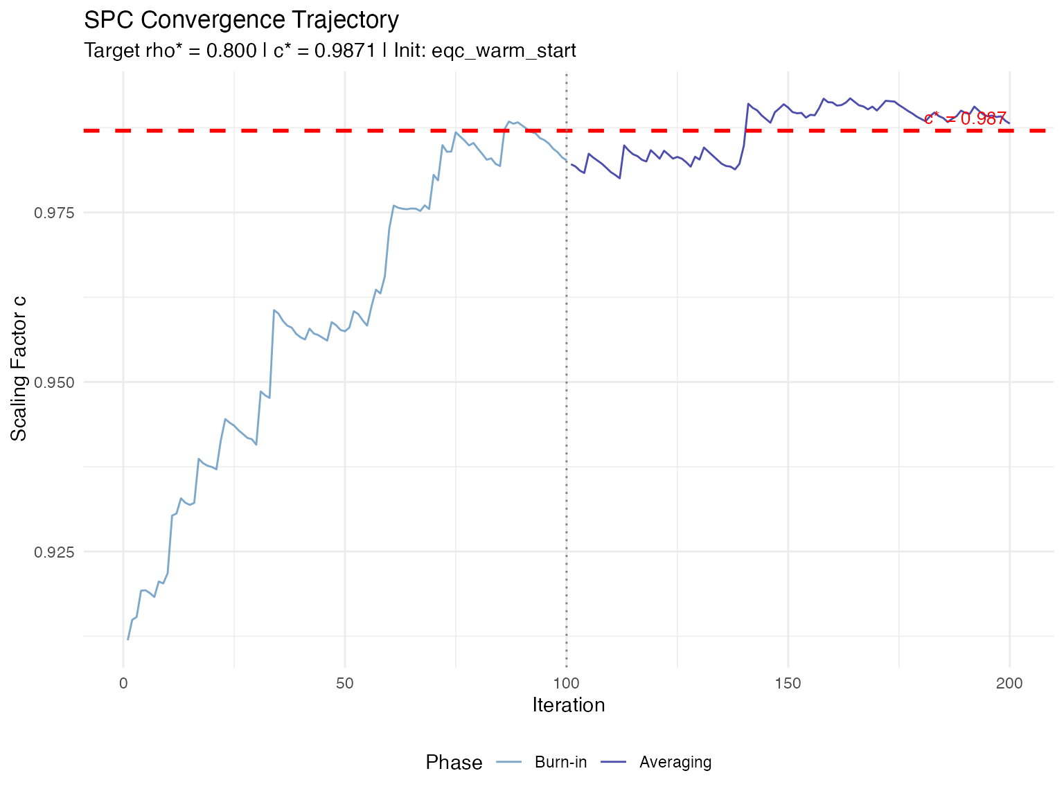

# Plot reliability estimates
plot(spc_result, type = "rho")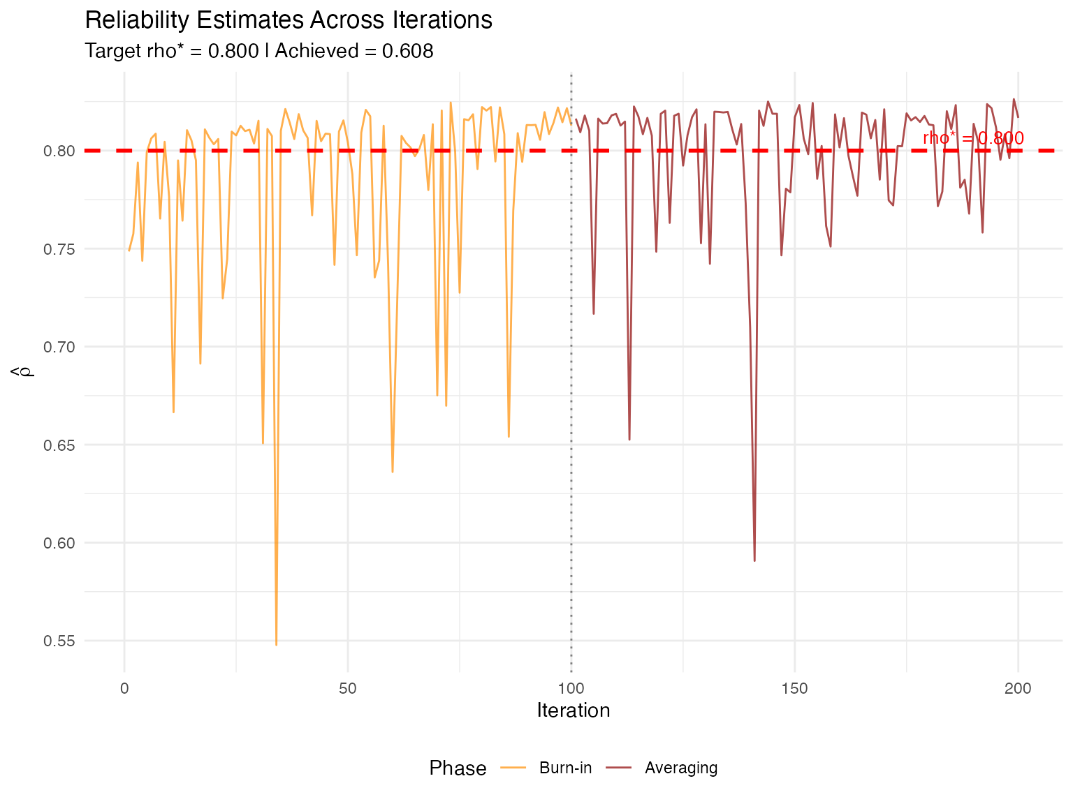

# Both plots combined (requires patchwork)
plot(spc_result, type = "both")

Key Parameters

Iteration Control

spc_result <- spc_calibrate(
  target_rho = 0.80,
  n_items = 25,
  n_iter = 300,       # Total iterations (default: 300)
  burn_in = 150,      # Discard first 150 for averaging (default: n_iter/2)
  seed = 42
)

Recommendations:

• n_iter = 200-300 is usually sufficient with warm start
• n_iter = 500+ for cold start or difficult problems
• burn_in should be at least 50% of n_iter

Monte Carlo Sample Sizes

spc_result <- spc_calibrate(
  target_rho = 0.80,
  n_items = 25,
  M_per_iter = 500,   # Samples per iteration (default: 500)
  M_pre = 10000,      # Samples for variance pre-calculation (default: 10000)
  seed = 42
)

Critical: M_pre controls the stability of the latent variance estimate $\sigma^2_\theta$, which is fixed throughout all iterations. Use M_pre >= 10000 for numerical stability.

Step Size Parameters

spc_result <- spc_calibrate(
  target_rho = 0.80,
  n_items = 25,
  step_params = list(
    a = 1.0,      # Base step size (default: 1.0)
    A = 50,       # Stabilization constant (default: 50)
    gamma = 0.67  # Decay exponent (default: 0.67 = 2/3)
  ),
  seed = 42
)

Guidance:

Situation	Adjustment
Slow convergence	Increase a
Oscillating trajectory	Decrease a or increase A
Too aggressive early steps	Increase A
Need faster decay	Increase gamma (max 1.0)

Item Resampling

# Resample item parameters each iteration (default)
spc_resample <- spc_calibrate(
  target_rho = 0.80,
  n_items = 25,
  resample_items = TRUE,
  seed = 42
)

# Fix item parameters across iterations
spc_fixed <- spc_calibrate(
  target_rho = 0.80,
  n_items = 25,
  resample_items = FALSE,
  seed = 42
)

• resample_items = TRUE: More robust, accounts for item parameter uncertainty
• resample_items = FALSE: Lower variance, faster convergence

Initialization Methods

SPC supports three initialization strategies:

1. EQC Warm Start (Recommended)

eqc_result <- eqc_calibrate(target_rho = 0.80, n_items = 25, seed = 42)

spc_result <- spc_calibrate(
  target_rho = 0.80,
  n_items = 25,
  c_init = eqc_result,  # Pass eqc_result object
  seed = 42
)
# init_method = "eqc_warm_start"

2. Analytic Pre-Calibration (APC)

When c_init = NULL, SPC uses a closed-form approximation:

spc_result <- spc_calibrate(
  target_rho = 0.80,
  n_items = 25,
  c_init = NULL,  # Uses APC warm start
  seed = 42
)
# init_method = "apc_warm_start"

The APC formula (under Gaussian Rasch assumptions):

$$c_{\text{init}} = \sqrt{\frac{\rho^*}{I \cdot \kappa \cdot (1 - \rho^*)}}$$

where $\kappa \approx 0.25 / \sqrt{1 + \sigma^2 \pi^2/3}$ is the logistic-normal convolution.

3. User-Specified Value

spc_result <- spc_calibrate(
  target_rho = 0.80,
  n_items = 25,
  c_init = 1.0,  # User-specified starting value
  seed = 42
)
# init_method = "user_specified"

Convergence Diagnostics

SPC provides automatic convergence assessment:

# Access convergence information
conv <- spc_result$convergence

cat("Convergence Diagnostics:\n")
#> Convergence Diagnostics:
cat(sprintf("  Converged: %s\n", conv$converged))
#>   Converged: TRUE
cat(sprintf("  Mean (first half):  %.4f\n", conv$mean_first_half))
#>   Mean (first half):  0.9842
cat(sprintf("  Mean (second half): %.4f\n", conv$mean_second_half))
#>   Mean (second half): 0.9900
cat(sprintf("  SD (post-burn-in):  %.4f\n", conv$sd_post_burn))
#>   SD (post-burn-in):  0.0037
cat(sprintf("  Final gradient:     %+.4f\n", conv$final_gradient))
#>   Final gradient:     +0.0167
cat(sprintf("  Hit lower bound:    %s\n", conv$hit_lower_bound))
#>   Hit lower bound:    FALSE
cat(sprintf("  Hit upper bound:    %s\n", conv$hit_upper_bound))
#>   Hit upper bound:    FALSE

Convergence Criteria

The algorithm is considered converged if:

$$|\bar{c}_{\text{first half}} - \bar{c}_{\text{second half}}| < 0.05$$

Handling Non-Convergence

If SPC doesn’t converge:

# Increase iterations
spc_result <- spc_calibrate(
  target_rho = 0.80,
  n_items = 25,
  n_iter = 500,     # More iterations
  burn_in = 250,
  seed = 42
)

# Adjust step sizes
spc_result <- spc_calibrate(
  target_rho = 0.80,
  n_items = 25,
  step_params = list(a = 0.5, A = 100, gamma = 0.67),  # Smaller, more stable steps
  seed = 42
)

# Use EQC warm start
eqc_result <- eqc_calibrate(target_rho = 0.80, n_items = 25, seed = 42)
spc_result <- spc_calibrate(
  target_rho = 0.80,
  n_items = 25,
  c_init = eqc_result,  # Start near solution
  n_iter = 150,         # Fewer iterations needed
  seed = 42
)

Understanding EQC vs SPC Differences

Why Do They Differ?

When comparing EQC and SPC results, you may notice systematic differences. This is expected and reflects theoretical distinctions:

EQC targets average-information reliability: $$\tilde{\rho}(c) = \frac{\sigma^2_\theta \bar{\mathcal{J}}(c)}{\sigma^2_\theta \bar{\mathcal{J}}(c) + 1}$$

SPC targets MSEM-based reliability (by default): $$\bar{\rho}(c) = \frac{\sigma^2_\theta}{\sigma^2_\theta + \mathbb{E}[1/\mathcal{J}(\theta; c)]}$$

Jensen’s inequality guarantees: $$\tilde{\rho}(c) \geq \bar{\rho}(c) \quad \text{for all } c$$

Therefore, to achieve the same target $\rho^*$:

$$c^*_{\text{SPC}} > c^*_{\text{EQC}}$$

Empirical Example

# Both targeting rho* = 0.80
eqc_result <- eqc_calibrate(
  target_rho = 0.80, n_items = 25,
  reliability_metric = "msem",  # Same metric
  seed = 42
)

spc_result <- spc_calibrate(
  target_rho = 0.80, n_items = 25,
  reliability_metric = "msem",  # Same metric
  c_init = eqc_result,
  seed = 42
)

# SPC's c* will be slightly higher
cat(sprintf("EQC c*: %.4f\n", eqc_result$c_star))
cat(sprintf("SPC c*: %.4f\n", spc_result$c_star))

Making Them Comparable

To maximize agreement, use the same reliability metric:

# Both use "info" metric
eqc_info <- eqc_calibrate(
  target_rho = 0.80, n_items = 25,
  reliability_metric = "info",
  seed = 42
)

spc_info <- spc_calibrate(
  target_rho = 0.80, n_items = 25,
  reliability_metric = "info",
  c_init = eqc_info,
  seed = 42
)

compare_eqc_spc(eqc_info, spc_info)

Verbose Mode

Enable detailed output to monitor progress:

# Level 1: Progress updates
spc_result <- spc_calibrate(
  target_rho = 0.80,
  n_items = 25,
  verbose = TRUE,   # or verbose = 1
  seed = 42
)

# Level 2: Iteration-by-iteration details
spc_result <- spc_calibrate(
  target_rho = 0.80,
  n_items = 25,
  verbose = 2,
  seed = 42
)

Working with Different Models

Rasch Model

spc_rasch <- spc_calibrate(
  target_rho = 0.75,
  n_items = 30,
  model = "rasch",
  seed = 42
)

2PL Model

spc_2pl <- spc_calibrate(
  target_rho = 0.80,
  n_items = 25,
  model = "2pl",
  item_source = "irw",
  item_params = list(
    discrimination_params = list(
      mu_log = 0,
      sigma_log = 0.3,
      rho = -0.3
    )
  ),
  seed = 42
)

Alias: sac_calibrate()

For nomenclature consistency with the manuscript, sac_calibrate() is provided as an alias:

# These are identical
spc_result <- spc_calibrate(target_rho = 0.80, n_items = 25, seed = 42)
sac_result <- sac_calibrate(target_rho = 0.80, n_items = 25, seed = 42)

Complete Validation Workflow

# ==== 1. Run EQC (primary calibration) ====
eqc_result <- eqc_calibrate(
  target_rho = 0.80,
  n_items = 25,
  model = "rasch",
  latent_shape = "normal",
  item_source = "irw",
  M = 20000,
  seed = 42,
  verbose = TRUE
)

# ==== 2. Validate with SPC ====
spc_result <- spc_calibrate(
  target_rho = 0.80,
  n_items = 25,
  model = "rasch",
  latent_shape = "normal",
  item_source = "irw",
  c_init = eqc_result,
  n_iter = 200,
  seed = 42,
  verbose = TRUE
)

# ==== 3. Compare results ====
comparison <- compare_eqc_spc(eqc_result, spc_result)

# ==== 4. Check convergence ====
if (!spc_result$convergence$converged) {
  warning("SPC did not converge. Consider increasing n_iter.")
}

# ==== 5. Visualize ====
plot(spc_result, type = "both")

# ==== 6. Final validation with TAM ====
sim_data <- simulate_response_data(
  eqc_result = eqc_result,
  n_persons = 1000,
  seed = 123
)

tam_rel <- compute_reliability_tam(sim_data$response_matrix, model = "rasch")

cat("\nFinal Validation Summary:\n")
cat(sprintf("  Target reliability:  %.3f\n", eqc_result$target_rho))
cat(sprintf("  EQC c*:              %.4f\n", eqc_result$c_star))
cat(sprintf("  SPC c*:              %.4f\n", spc_result$c_star))
cat(sprintf("  Agreement:           %.2f%%\n", comparison$diff_pct))
cat(sprintf("  TAM WLE reliability: %.3f\n", tam_rel$rel_wle))
cat(sprintf("  TAM EAP reliability: %.3f\n", tam_rel$rel_eap))

Troubleshooting Guide

Problem	Cause	Solution
Slow convergence	Poor initialization	Use EQC warm start
Oscillating trajectory	Step size too large	Decrease a, increase A
Hitting bounds	Target outside feasible range	Extend c_bounds
High post-burn-in SD	Insufficient averaging	Increase n_iter
Divergence	Step size too aggressive	Use gamma = 0.75 or higher
Memory issues	Large M_per_iter	Reduce to 300-500

Theoretical Properties

Convergence Guarantee

Under standard Robbins-Monro conditions, the SPC iterate converges almost surely:

$$c_n \xrightarrow{\text{a.s.}} c^* \quad \text{as } n \to \infty$$

Asymptotic Normality

With Polyak-Ruppert averaging:

$$\sqrt{n}(c^*_n - c^*) \xrightarrow{d} N(0, \sigma^2 / g'(c^*)^2)$$

where $\sigma^2$ is the variance of the gradient noise and $g'(c^*)$ is the derivative of the reliability function at the solution.

Rate of Convergence

• Final iterate: $O(n^{-\gamma})$ convergence
• Polyak-Ruppert average: $O(n^{-1/2})$ convergence (optimal rate)

Summary

SPC is a flexible, theoretically-grounded algorithm for reliability-targeted calibration:

• Best practice: Use EQC for primary calibration, SPC for validation
• Warm start: Always use EQC result when available
• Convergence: Check spc_result$convergence$converged
• Visualization: Use plot(spc_result) to inspect trajectory
• Differences from EQC: Expected due to reliability metric definitions

For routine simulation work, EQC alone is typically sufficient. Use SPC when you need independent validation or are working with complex scenarios where EQC’s assumptions may not hold.

References

Robbins, H., & Monro, S. (1951). A stochastic approximation method. The Annals of Mathematical Statistics, 22(3), 400–407.

Polyak, B. T., & Juditsky, A. B. (1992). Acceleration of stochastic approximation by averaging. SIAM Journal on Control and Optimization, 30(4), 838–855.

Kushner, H. J., & Yin, G. G. (2003). Stochastic Approximation and Recursive Algorithms and Applications (2nd ed.). Springer.