
Simulation Study: Evaluating Prior Models and Posterior Summaries
JoonHo Lee
2026-07-23
Source:vignettes/simulation-study.Rmd
simulation-study.RmdOverview
Simulation studies are the primary tool for evaluating IRT methods because they provide access to the ground truth — the true person abilities and item parameters that generated the data. DPMirt provides an integrated simulation framework that lets you:
- Simulate data under known conditions using IRTsimrel calibration for Rasch/2PL models, or DPMirt’s built-in fallback.
- Fit models under competing prior specifications (Normal vs. DPM).
- Estimate person abilities using three posterior summary methods (PM, CB, GR).
- Evaluate performance using multiple loss functions (MSEL, MSELR, KS).
This vignette walks through a complete simulation study design, executes a single-condition deep dive, interprets the results, and provides templates for scaling to a full factorial study.
Simulation Design
The APM manuscript (Lee & Wind) uses a factorial design crossing three factors:
Factor 1: Latent Distribution Shape ()
| Shape | Description | Generating mechanism |
|---|---|---|
| Normal | Standard Gaussian | |
| Bimodal | Two-group mixture | |
| Skew | Right-skewed | Shifted exponential: |
The Normal condition is the parametric model’s “home turf” where DPM offers little advantage. The Bimodal and Skew conditions represent departures where flexible priors may help, especially for distributional summaries.
Factor 2: Sample Size ()
| Interpretation | |
|---|---|
| 50 | Small sample: high uncertainty, strong shrinkage |
| 200 | Moderate sample: reliable estimation for most methods |
Factor 3: Marginal Reliability ()
Reliability is the most influential factor in the simulation. It controls the information per person and therefore the degree of posterior shrinkage.
| w-bar | ~Items (Rasch) | Shrinkage | Separation |
|---|---|---|---|
| 0.50 | ~10 | Severe | 1.0 |
| 0.70 | ~23 | Moderate | 1.5 |
| 0.90 | ~61 | Mild | 3.0 |
Why reliability dominates: At , each person’s posterior is heavily shrunk toward the prior, so prior differences are harder to see and estimator choice can dominate distributional recovery. At , posteriors are tightly concentrated around data-driven estimates, making prior misspecification easier to detect.
Full Design Matrix
The full factorial design has conditions. Each condition is replicated (e.g., 100 times) for Monte Carlo stability.
| Condition | G | N | w_bar |
|---|---|---|---|
| 1 | Normal | 50 | 0.5 |
| 2 | Bimodal | 50 | 0.5 |
| 3 | Skew | 50 | 0.5 |
| 4 | Normal | 200 | 0.5 |
| 5 | Bimodal | 200 | 0.5 |
| 6 | Skew | 200 | 0.5 |
| 7 | Normal | 50 | 0.7 |
| 8 | Bimodal | 50 | 0.7 |
| 9 | Skew | 50 | 0.7 |
| 10 | Normal | 200 | 0.7 |
| 11 | Bimodal | 200 | 0.7 |
| 12 | Skew | 200 | 0.7 |
| 13 | Normal | 50 | 0.9 |
| 14 | Bimodal | 50 | 0.9 |
| 15 | Skew | 50 | 0.9 |
| 16 | Normal | 200 | 0.9 |
| 17 | Bimodal | 200 | 0.9 |
| 18 | Skew | 200 | 0.9 |
IRTsimrel Integration
DPMirt uses the IRTsimrel package (when available)
to achieve precise reliability targeting for Rasch and 2PL simulations.
The default average-information metric uses Empirical Quadrature
Calibration (EQC); MSEM-based targets use IRTsimrel’s SAC calibration.
The key function is dpmirt_simulate():
# Simulate bimodal data with target reliability 0.8
sim <- dpmirt_simulate(
  n_persons    = 200,
  n_items      = 25,
  model        = "rasch",
  target_rho   = 0.8,
  latent_shape = "bimodal",
  seed         = 42
)

sim
#> DPMirt Simulated Data
#> =====================
#> Model:         RASCH
#> Persons:       200
#> Items:         25
#> Distribution:  bimodal
#> Method:        irtsimrel
#> Target rho:    0.8
#> KR-20:         0.798
#> EQC c*:       0.9356
#> EQC rho:      0.8
The returned dpmirt_sim object reports:
- Method: “irtsimrel” (IRTsimrel-calibrated) or “fallback” (Paganin-style)
- KR-20: Empirical reliability of the generated data
-
Achieved rho: IRTsimrel calibration-level achieved
marginal reliability (
sim$achieved_rho) when IRTsimrel was used;NULLfor fallback simulations -
Target rho: the requested reliability when
IRTsimrel was used;
NULLfor fallback simulations - Calibration c*: the calibration constant when IRTsimrel was used
When IRTsimrel is not installed, or when model = "3pl",
dpmirt_simulate() falls back to a simpler simulation with
evenly spaced item difficulties and no reliability targeting. 3PL
fallback simulations include Beta-distributed guessing parameters
delta, and target_rho is not used.
Visualizing the Simulated Data
theta_dens <- density(sim$theta)
plot(theta_dens, main = "True theta distribution (bimodal)",
     xlab = expression(theta), lwd = 2)
rug(sim$theta, col = adjustcolor("black", alpha.f = 0.2))
Density of true theta values from the bimodal simulation.
sum_scores <- rowSums(sim$response)
hist(sum_scores, breaks = 20, main = "Sum score distribution",
     xlab = "Sum score", col = adjustcolor(pal$parametric, alpha.f = 0.5),
     border = "white")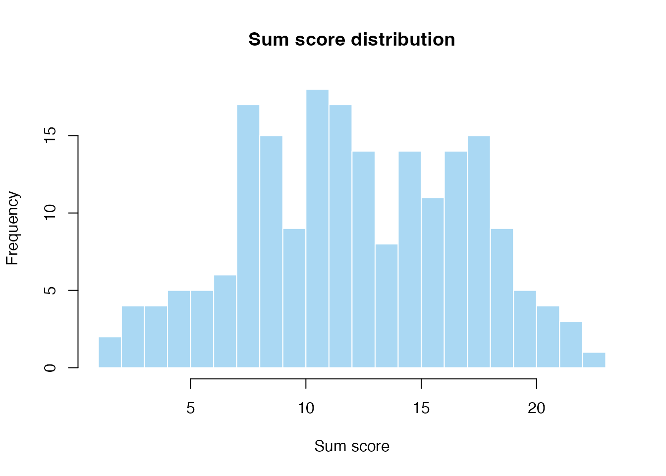
Distribution of sum scores from the simulated response matrix.
Analysis Pipeline
The full analysis pipeline for a single simulation condition consists of six steps. Below we show the complete code you would run in a live session, then load pre-computed results for the remaining analysis.
Step 1: Simulate Data
sim <- dpmirt_simulate(
  n_persons    = 200,
  n_items      = 25,
  model        = "rasch",
  target_rho   = 0.8,
  latent_shape = "bimodal",
  seed         = 42
)
Step 2: Fit Models
# --- Fit Normal prior model (~2 min compilation + sampling) ---
fit_normal <- dpmirt(
  sim$response,
  model   = "rasch",
  prior   = "normal",
  niter   = 10000,
  nburnin = 2000,
  thin    = 32,
  thin2   = 32,
  seed    = 100
)

# --- Fit DPM prior model (~2 min compilation + sampling) ---
# Bundled fixtures use the conservative Gamma(1,3) alpha prior.
fit_dpm <- dpmirt(
  sim$response,
  model   = "rasch",
  prior   = "dpm",
  niter   = 10000,
  nburnin = 2000,
  thin    = 32,
  thin2   = 32,
  seed    = 101
)
Step 3: Extract Estimates
# Compute PM, CB, GR for both models
est_normal <- dpmirt_estimates(fit_normal, methods = c("pm", "cb", "gr"))
est_dpm    <- dpmirt_estimates(fit_dpm,    methods = c("pm", "cb", "gr"))
Step 4: Evaluate Losses
# Compare to true theta
loss_normal <- dpmirt_loss(est_normal, true_theta = sim$theta,
                            true_beta = sim$beta)
loss_dpm    <- dpmirt_loss(est_dpm,    true_theta = sim$theta,
                            true_beta = sim$beta)
Step 5: Combine Results
loss_normal$prior <- "Normal"
loss_dpm$prior    <- "DPM"
combined_loss <- rbind(loss_normal, loss_dpm)
Loading Pre-Computed Results
For this vignette, all fitting results are pre-computed: the bundled DPM fixtures use the conservative prior for , so the example does not require DPprior.
# Load pre-computed simulation data
sim_data <- readRDS(find_extdata("vignette_sim_bimodal.rds"))

# Load estimates comparison (all 6 method-prior combos)
est_comparison <- readRDS(find_extdata("vignette_estimates_comparison.rds"))

# Load loss results
loss_results <- readRDS(find_extdata("vignette_loss_results.rds"))
Single Condition Deep Dive
We focus on the most informative condition: Bimodal, , . This condition is useful because the true latent distribution violates the Gaussian assumption while the data are informative enough to compare posterior summaries. In the bundled fixture, the DPM prior has its clearest edge on the KS distributional loss, while Normal-prior GR is slightly better on the rank loss.
Posterior Density Overlay
theta_true <- est_comparison$true_theta
N <- length(theta_true)

df_dens <- data.frame(
  value = c(theta_true,
            est_comparison$normal$theta$theta_pm,
            est_comparison$normal$theta$theta_cb,
            est_comparison$normal$theta$theta_gr,
            est_comparison$dpm$theta$theta_pm,
            est_comparison$dpm$theta$theta_cb,
            est_comparison$dpm$theta$theta_gr),
  Method = factor(rep(c("True", "Normal-PM", "Normal-CB", "Normal-GR",
                         "DPM-PM", "DPM-CB", "DPM-GR"), each = N),
                  levels = c("True", "Normal-PM", "Normal-CB", "Normal-GR",
                             "DPM-PM", "DPM-CB", "DPM-GR"))
)

method_colors <- c(
  "True"      = "black",
  "Normal-PM" = pal$normal_pm, "Normal-CB" = pal$normal_cb,
  "Normal-GR" = pal$normal_gr,
  "DPM-PM"    = pal$dpm_pm, "DPM-CB" = pal$dpm_cb,
  "DPM-GR"    = pal$dpm_gr
)
method_lty <- c("True" = "solid",
                "Normal-PM" = "solid", "Normal-CB" = "dashed",
                "Normal-GR" = "dotted",
                "DPM-PM"    = "solid", "DPM-CB"    = "dashed",
                "DPM-GR"    = "dotted")

ggplot(df_dens, aes(x = value, colour = Method, linetype = Method)) +
  geom_density(linewidth = 0.9, fill = NA) +
  scale_colour_manual(values = method_colors) +
  scale_linetype_manual(values = method_lty) +
  labs(title = "Posterior density comparison: 6 methods vs. truth",
       subtitle = "Bimodal population, 25 items, 200 persons",
       x = expression(theta), y = "Density") +
  theme_bw() +
  theme(legend.position = "right")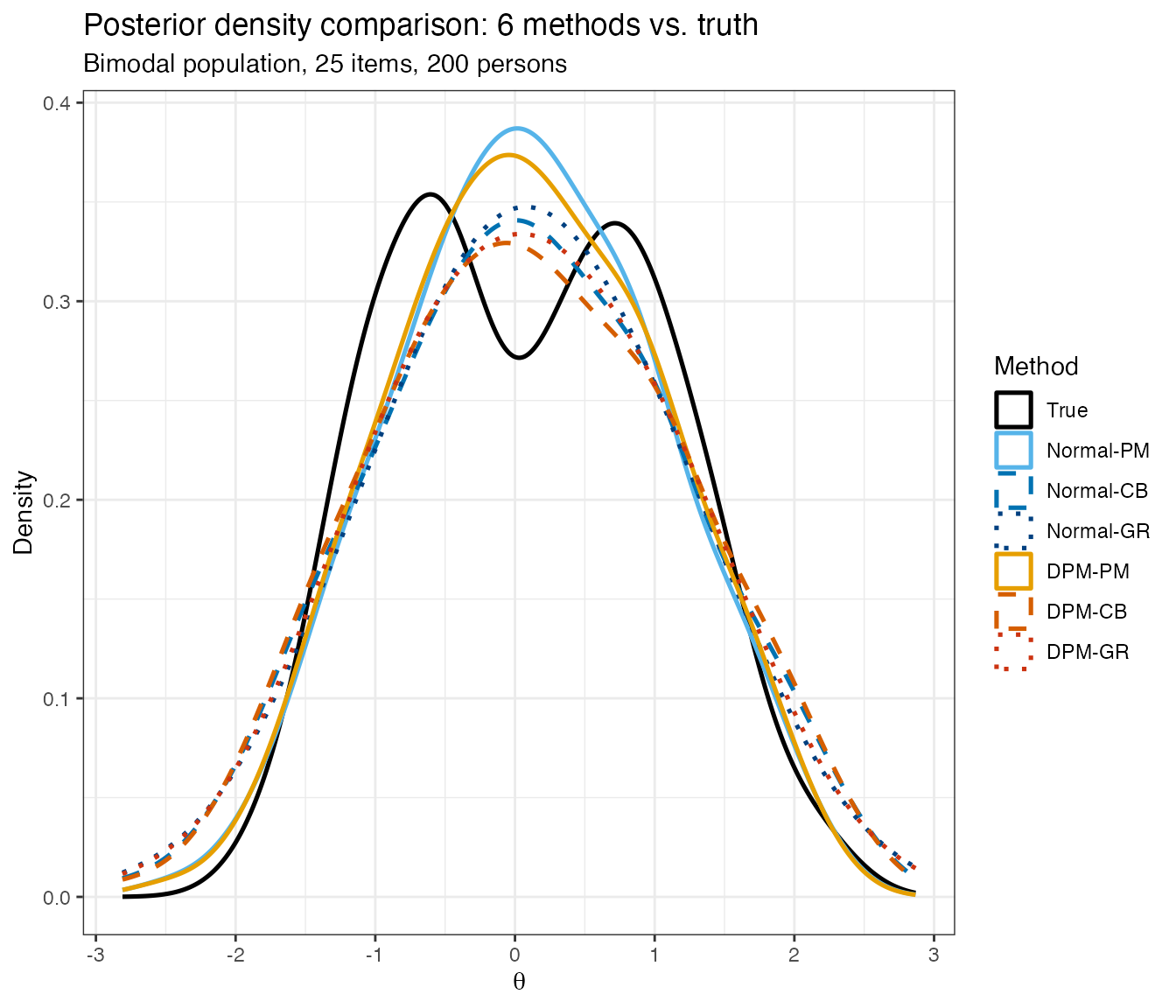
Density estimates from six method-prior combinations overlaid with the true latent density. In this fixture, DPM-GR gives the smallest KS loss while posterior means remain visibly shrunk.
What to look for: Posterior means are visibly compressed under both priors. CB and GR de-shrink the estimates, and in this fixture DPM-GR has the smallest KS distance to the true distribution. Ranking and individual MSE should be read from the loss table rather than inferred from the density alone.
Shrinkage Comparison
par(mfrow = c(1, 2))

# Normal-PM
plot(theta_true, est_comparison$normal$theta$theta_pm,
     pch = 16, cex = 0.6, col = adjustcolor(pal$normal_pm, 0.6),
     xlab = expression(theta[true]), ylab = expression(hat(theta)[PM]),
     main = "Normal-PM", asp = 1)
abline(0, 1, col = pal$reference, lwd = 1.5, lty = 2)

# DPM-PM
plot(theta_true, est_comparison$dpm$theta$theta_pm,
     pch = 16, cex = 0.6, col = adjustcolor(pal$dpm_pm, 0.6),
     xlab = expression(theta[true]), ylab = expression(hat(theta)[PM]),
     main = "DPM-PM", asp = 1)
abline(0, 1, col = pal$reference, lwd = 1.5, lty = 2)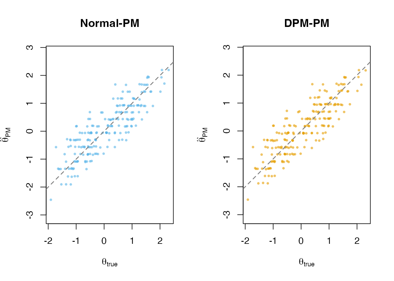
Posterior mean (PM) estimates vs. true theta. PM estimates are shrunk toward the center under both priors in this fixture.
Loss Function Results
Three complementary loss functions capture different aspects of estimator quality:
| Loss | Formula | Measures |
|---|---|---|
| MSEL | Individual accuracy (Goal 1) | |
| MSELR | Ranking accuracy (Goal 2) | |
| KS | Distributional fidelity (Goal 3) |
# loss_results is a list with $normal and $dpm data.frames,
# each with columns: parameter, method, msel, mselr, ks

# Combine into one table with a prior column
loss_normal <- loss_results$normal
loss_normal$prior <- "Normal"
loss_dpm <- loss_results$dpm
loss_dpm$prior <- "DPM"
loss_combined <- rbind(loss_normal, loss_dpm)

# Filter to theta and format
loss_display <- loss_combined[loss_combined$parameter == "theta", ]
loss_display <- loss_display[order(loss_display$prior, loss_display$method), ]

loss_display$Label <- paste0(loss_display$prior, "-",
                              toupper(loss_display$method))
loss_display <- loss_display[, c("Label", "msel", "mselr", "ks")]
names(loss_display) <- c("Method", "MSEL", "MSELR", "KS")
loss_display$MSEL  <- round(loss_display$MSEL, 4)
loss_display$MSELR <- round(loss_display$MSELR, 5)
loss_display$KS    <- round(loss_display$KS, 4)

knitr::kable(loss_display, row.names = FALSE,
             caption = "Loss function results: Bimodal, N=200, w-bar=0.8.",
align = "lccc")| Method | MSEL | MSELR | KS |
|---|---|---|---|
| DPM-CB | 0.3029 | 0.02499 | 0.080 |
| DPM-GR | 0.3136 | 0.02487 | 0.055 |
| DPM-PM | 0.2544 | 0.02499 | 0.095 |
| Normal-CB | 0.3010 | 0.02460 | 0.090 |
| Normal-GR | 0.3057 | 0.02439 | 0.060 |
| Normal-PM | 0.2544 | 0.02460 | 0.095 |
Interpreting the Loss Table
# Identify best method for each loss
best_msel  <- loss_display$Method[which.min(loss_display$MSEL)]
best_mselr <- loss_display$Method[which.min(loss_display$MSELR)]
best_ks    <- loss_display$Method[which.min(loss_display$KS)]

cat("Best for MSEL  (individual accuracy):", best_msel, "\n")
#> Best for MSEL  (individual accuracy): DPM-PM
cat("Best for MSELR (ranking accuracy):   ", best_mselr, "\n")
#> Best for MSELR (ranking accuracy):    Normal-GR
cat("Best for KS    (distributional):     ", best_ks, "\n")
#> Best for KS    (distributional):      DPM-GR
Visual Loss Comparison
method_colors_vec <- c(
  "Normal-CB" = pal$normal_cb, "Normal-GR" = pal$normal_gr,
  "Normal-PM" = pal$normal_pm,
  "DPM-CB"    = pal$dpm_cb, "DPM-GR" = pal$dpm_gr,
  "DPM-PM"    = pal$dpm_pm
)

loss_long <- data.frame(
  Method = rep(loss_display$Method, 3),
  Metric = rep(c("MSEL", "MSELR", "KS"), each = nrow(loss_display)),
  Loss   = c(loss_display$MSEL, loss_display$MSELR, loss_display$KS)
)
loss_long$Method <- factor(loss_long$Method, levels = loss_display$Method)
loss_long$Metric <- factor(loss_long$Metric, levels = c("MSEL", "MSELR", "KS"))

ggplot(loss_long, aes(x = Method, y = Loss, fill = Method)) +
  geom_col(width = 0.7) +
  facet_wrap(~ Metric, scales = "free_y", ncol = 3) +
  scale_fill_manual(values = method_colors_vec, guide = "none") +
  labs(title = "Loss comparison: 6 method-prior combinations",
       y = "Loss (lower is better)") +
  theme_bw() +
  theme(axis.text.x = element_text(angle = 45, hjust = 1, size = 9),
        strip.text = element_text(face = "bold", size = 11))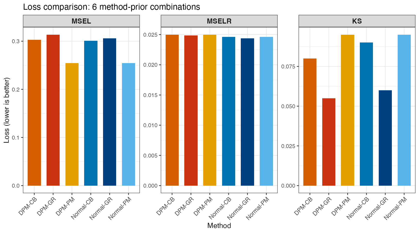
Bar chart of loss values across six methods. Lower is better for all three metrics; the best prior-method combination differs by metric.
Low-Reliability Contrast
The deep dive above used a 25-item test () where the data are informative enough to compare prior and estimator choices. How do the patterns change when reliability is much lower?
comp_hi <- est_comparison
comp_lo <- readRDS(find_extdata("vignette_estimates_comparison_lowrel.rds"))

build_panel <- function(comp_obj, label) {
  N <- length(comp_obj$true_theta)
  data.frame(
    value = c(comp_obj$true_theta,
              comp_obj$dpm$theta$theta_pm,
              comp_obj$dpm$theta$theta_cb,
              comp_obj$dpm$theta$theta_gr),
    Method = factor(rep(c("True", "DPM-PM", "DPM-CB", "DPM-GR"), each = N),
                    levels = c("True", "DPM-PM", "DPM-CB", "DPM-GR")),
    Reliability = label
  )
}

df_rel <- rbind(
  build_panel(comp_lo, "\u03C1 \u2248 0.5  (10 items)"),
  build_panel(comp_hi, "\u03C1 \u2248 0.8  (25 items)")
)
df_rel$Reliability <- factor(df_rel$Reliability,
  levels = c("\u03C1 \u2248 0.5  (10 items)",
             "\u03C1 \u2248 0.8  (25 items)"))

rel_colors <- c("True" = "gray40", "DPM-PM" = pal$dpm_pm,
                "DPM-CB" = pal$dpm_cb, "DPM-GR" = pal$dpm_gr)

ggplot(df_rel, aes(x = value, colour = Method, fill = Method)) +
  geom_density(alpha = 0.12, linewidth = 0.9) +
  facet_wrap(~ Reliability, ncol = 2) +
  scale_colour_manual(values = rel_colors) +
  scale_fill_manual(values = rel_colors) +
  labs(title = "Reliability determines when estimator choice matters",
       x = expression(theta), y = "Density") +
  theme_bw() +
  theme(legend.position = "top",
        strip.text = element_text(face = "bold", size = 11))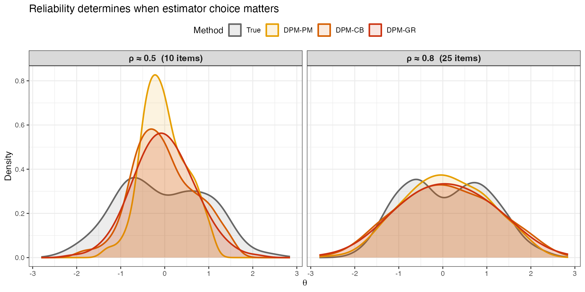
Posterior density comparison at two reliability levels (DPM prior only). Left (, 10 items): severe shrinkage compresses PM toward the center, while CB and GR recover more spread. Right (, 25 items): shrinkage is milder and the estimators move closer together.
| Reliability | Method | MSEL | MSELR | KS |
|---|---|---|---|---|
| ρ ≈ 0.5 | PM | 0.5561 | 0.054310 | 0.285 |
| ρ ≈ 0.5 | CB | 0.5234 | 0.054310 | 0.220 |
| ρ ≈ 0.5 | GR | 0.5338 | 0.054209 | 0.165 |
| ρ ≈ 0.8 | PM | 0.2544 | 0.024992 | 0.095 |
| ρ ≈ 0.8 | CB | 0.3029 | 0.024992 | 0.080 |
| ρ ≈ 0.8 | GR | 0.3136 | 0.024868 | 0.055 |
Key observation. At , the choice of estimator (PM vs. CB vs. GR) matters more than the choice of prior, because every person’s posterior is heavily shrunk toward the prior center. CB and GR resist this compression, producing estimates whose distribution more closely tracks the truth. In this bundled low-reliability fixture, CB and GR also improve MSEL relative to PM, so the direction of the MSEL tradeoff should be checked empirically rather than assumed.
Dispersion Recovery at Two Reliability Levels
| Reliability | SD(True) | SD(PM) | SD(CB) | SD(GR) | PM/True | GR/True |
|---|---|---|---|---|---|---|
| ρ ≈ 0.5 | 0.991 | 0.493 | 0.700 | 0.696 | 0.50 | 0.70 |
| ρ ≈ 0.8 | 0.955 | 0.948 | 1.075 | 1.073 | 0.99 | 1.12 |
Pattern. At low reliability, PM compresses the ability distribution to roughly half its true spread (PM/True ), effectively destroying the bimodal structure. The GR estimator retains about 70% of the true dispersion (GR/True ), substantially reducing the information loss. At high reliability, the estimators move closer to the true spread, though shrinkage and prior effects should still be checked with the relevant loss metric.
Key Patterns
The simulation study from Lee & Wind reveals four main findings:
Finding 1: Reliability Dominates Over Sample Size
Across all conditions, the marginal reliability is a stronger predictor of estimator performance than sample size . At , prior-family differences are harder to distinguish because the data are weak; estimator choice can still matter for distributional loss. At , prior-family and estimator differences can become easier to see.
Implication: Invest in longer tests (more items) rather than larger samples if your goal is to discriminate between Normal and DPM priors.
Finding 2: DPM Can Help Under Non-Normality + Sufficient Reliability
The DPM prior is most likely to help when:
- The true latent distribution is non-normal (bimodal or skewed), and
- Reliability is at least moderate ().
Under normality, the DPM prior performs comparably to the Normal prior — the DP adapts to the true distribution and does not distort it.
Finding 3: Match the Estimator to the Loss
The three posterior summary methods optimize different goals:
| Method | Strength | When to use |
|---|---|---|
| PM | Targets individual MSE (MSEL) | Point predictions for each person |
| CB | Better distributional match than PM | Group-level summary statistics |
| GR | Lowest KS distance | Percentile reports, distributional inference |
PM is the traditional choice for Goal 1 (minimizing per-person squared error), though finite-sample fixtures can occasionally favor a de-shrunk estimator on MSEL. However, PM tends to over-shrink toward the prior center, producing estimates whose empirical distribution is too narrow when distributional recovery is the goal.
CB and GR “de-shrink” the estimates to better match the true distribution, often at a cost to individual MSE, but the realized tradeoff should be read from the loss table.
Finding 4: No One-Size-Fits-All
No single method–prior combination dominates across all conditions and loss functions simultaneously. The optimal choice depends on:
- The shape of the true latent distribution (or your best guess).
- The reliability of the instrument.
- The inferential goal (individual prediction vs. distributional reporting).
Recommendation: For routine use, fit both Normal and DPM models, compare predictive fit with WAIC, inspect posterior-summary densities, and select the estimator (PM, CB, or GR) that matches your reporting goals. WAIC evaluates item-response prediction, not ability-distribution recovery.
Scaling to a Full Study
The single-condition pipeline above can be wrapped in a loop for a full Monte Carlo study. Below is a template that you would run in a non-interactive session (e.g., on a computing cluster). This code is shown but not executed in the vignette:
# ============================================================
# Full simulation study template
# ============================================================
# WARNING: This runs 18 conditions x 100 replications x 2 models
# Estimated time: ~72 hours on a single core
# ============================================================

library(DPMirt)

if (!requireNamespace("IRTsimrel", quietly = TRUE)) {
  stop(
    "This template uses IRTsimrel reliability targeting and the 'skew_pos' ",
    "latent-shape name. Install IRTsimrel, or replace 'skew_pos' with ",
    "'skewed' and remove reliability-targeting assumptions."
  )
}

# --- Design ---
conditions <- expand.grid(
  latent_shape = c("normal", "bimodal", "skew_pos"),
  n_persons    = c(50, 200),
  target_rho   = c(0.5, 0.7, 0.9),
  stringsAsFactors = FALSE
)

n_reps  <- 100
n_items <- 25

# --- Storage ---
all_results <- vector("list", nrow(conditions) * n_reps)
result_idx  <- 0

for (cond in seq_len(nrow(conditions))) {
  cfg <- conditions[cond, ]
  cat("Condition", cond, "/", nrow(conditions), ":",
      cfg$latent_shape, "N =", cfg$n_persons,
      "rho =", cfg$target_rho, "\n")

  for (rep in seq_len(n_reps)) {
    result_idx <- result_idx + 1
    rep_seed   <- cond * 1000 + rep

    # --- Step 1: Simulate ---
    sim <- dpmirt_simulate(
      n_persons    = cfg$n_persons,
      n_items      = n_items,
      model        = "rasch",
      target_rho   = cfg$target_rho,
      latent_shape = cfg$latent_shape,
      seed         = rep_seed
    )

    if (!identical(sim$method, "irtsimrel")) {
      stop("Expected IRTsimrel simulation for this reliability-targeted study.")
    }

    # --- Step 2: Fit Normal ---
    fit_n <- dpmirt(
      sim$response,
      model   = "rasch",
      prior   = "normal",
      niter   = 10000,
      nburnin = 2000,
      seed    = rep_seed + 1,
      verbose = FALSE
    )

    # --- Step 3: Fit DPM ---
    fit_d <- dpmirt(
      sim$response,
      model   = "rasch",
      prior   = "dpm",
      niter   = 10000,
      nburnin = 2000,
      seed    = rep_seed + 2,
      verbose = FALSE
    )

    # --- Step 4: Estimate ---
    est_n <- dpmirt_estimates(fit_n, methods = c("pm", "cb", "gr"))
    est_d <- dpmirt_estimates(fit_d, methods = c("pm", "cb", "gr"))

    # --- Step 5: Evaluate ---
    loss_n <- dpmirt_loss(est_n, true_theta = sim$theta,
                           true_beta = sim$beta)
    loss_d <- dpmirt_loss(est_d, true_theta = sim$theta,
                           true_beta = sim$beta)

    loss_n$prior <- "Normal"
    loss_d$prior <- "DPM"

    # --- Step 6: Store ---
    all_results[[result_idx]] <- cbind(
      rbind(loss_n, loss_d),
      condition    = cond,
      replication  = rep,
      latent_shape = cfg$latent_shape,
      n_persons    = cfg$n_persons,
      target_rho   = cfg$target_rho,
      achieved_rho = sim$achieved_rho,
      waic_normal  = fit_n$waic,
      waic_dpm     = fit_d$waic,
      reliability  = sim$reliability
    )
  }
}

# --- Combine ---
results_df <- do.call(rbind, all_results)

# --- Save ---
saveRDS(results_df, "simulation_results.rds")
Parallelization
For faster execution, parallelize across conditions using
parallel::mclapply() or a cluster scheduler:
library(parallel)

run_one_condition <- function(cond, n_reps = 100) {
  cfg <- conditions[cond, ]
  # ... same inner loop as above ...
}

# Run on 4 cores (adjust to your machine)
results_list <- mclapply(
  seq_len(nrow(conditions)),
  run_one_condition,
  mc.cores = 4
)
This template assumes IRTsimrel is installed for Rasch reliability
targeting and for the skew_pos latent-shape name. Without
IRTsimrel, DPMirt uses the fallback simulator, ignores
target_rho, and supports the fallback shape names
"normal", "bimodal", and
"skewed".
Extending the Study
The DPMirt simulation framework supports several extensions beyond the basic Rasch study:
2PL Models
sim_2pl <- dpmirt_simulate(
  n_persons    = 200,
  n_items      = 25,
  model        = "2pl",
  target_rho   = 0.8,
  latent_shape = "bimodal",
  seed         = 42
)

fit_2pl <- dpmirt(
  sim_2pl$response,
  model = "2pl",
  prior = "dpm",
  niter = 15000,
  nburnin = 3000
)
Custom Latent Distributions
With IRTsimrel installed, you have access to 12 distribution shapes:
# Built-in supported shapes (when IRTsimrel is available)
shapes <- c("normal", "bimodal", "trimodal", "multimodal",
            "skew_pos", "skew_neg", "heavy_tail", "light_tail",
            "uniform", "floor", "ceiling")

for (shape in shapes) {
  sim <- dpmirt_simulate(200, 25, latent_shape = shape, seed = 42)
  cat(shape, ": KR-20 =", round(sim$reliability, 3), "\n")
}

# Custom shapes require IRTsimrel, a Rasch or 2PL simulation,
# and latent_params = list(mixture_spec = ...).
custom_sim <- dpmirt_simulate(
  200, 25,
  latent_shape  = "custom",
  latent_params = list(mixture_spec = list(
    weights = c(0.5, 0.5),
    means   = c(-1, 1),
    sds     = c(0.5, 0.5)
  )),
  seed          = 42
)
Custom latent distributions are not available in fallback simulation or for 3PL.
Custom Loss Functions
Extend evaluation with your own loss function:
# Bias (signed error)
bias_loss <- function(estimate, true) mean(estimate - true)

# Coverage of 95% CI
coverage_loss <- function(estimate, true) {
  # Requires access to full posterior...
  # Use dpmirt_draws() for this
}

loss_custom <- dpmirt_loss(
  est_dpm,
  true_theta  = sim$theta,
  custom_loss = bias_loss
)
Diagnostic Checks for Simulation Validity
Before interpreting results, verify that the simulation and MCMC converged properly.
Check 1: Achieved Reliability
cat("Target reliability:", 0.8, "\n")
#> Target reliability: 0.8
cat("Empirical KR-20: ", round(sim$reliability, 4), "\n")
#> Empirical KR-20:  0.7983
if (!is.null(sim$achieved_rho)) {
  cat("Calibration rho: ", round(sim$achieved_rho, 4), "\n")
}
#> Calibration rho:  0.8
cat("Simulation method: ", sim$method, "\n")
#> Simulation method:  irtsimrel
Check 2: MCMC Convergence
For pre-computed fits, you would check:
# Minimum ESS across all parameters
min(fit$ess$items)   # Review relative to retained thinned draws
min(fit$ess$theta)

# Trace plot
plot(fit, type = "trace")

# WAIC comparison
cat("WAIC Normal:", fit_normal$waic, "\n")
cat("WAIC DPM:   ", fit_dpm$waic, "\n")
For the bundled compact fixtures, ESS is computed from 250 retained thinned draws and is intended for documentation-scale screening. Use full simulation runs, with many more retained draws, for convergence assessment in a study.
Check 3: Posterior Predictive Check
# Compare observed vs. predicted sum score distribution
plot(fit, type = "pp_check")
Summary Table of Functions
| Function | Purpose | Phase |
|---|---|---|
dpmirt_simulate() |
Generate IRT data; target reliability for Rasch/2PL when IRTsimrel is available | Simulation |
dpmirt() |
Fit model (one-step) | Fitting |
dpmirt_estimates() |
Compute PM, CB, GR estimates | Estimation |
dpmirt_loss() |
Evaluate MSEL, MSELR, KS | Evaluation |
dpmirt_draws() |
Extract retained rescaled posterior draws | Post-hoc analysis |
dpmirt_dp_density() |
Compute DP mixture density | DPM diagnostics |
What’s Next?
| Vignette | Why read it |
|---|---|
| Quick Start | Simpler walkthrough of the basic pipeline |
| Prior Elicitation | Optional DPprior calibration of and Gamma(1,3) fallback |
| NIMBLE Internals | NIMBLE internals, live compile-once pattern, custom sampler hooks |
References
Lee, J. & Wind, S. Targeting toward inferential goals in Bayesian Rasch models for estimating person-specific latent traits. OSF Preprint. https://doi.org/10.31219/osf.io/qrw4n
Lee, J. (2025). Reliability-targeted simulation of item response data: Solving the inverse design problem. arXiv preprint arXiv:2512.16012. https://arxiv.org/abs/2512.16012
Paganin, S., Paciorek, C. J., Wehrhahn, C., Rodríguez, A., Rabe-Hesketh, S., & de Valpine, P. (2023). Computational strategies and estimation performance with Bayesian semiparametric item response theory models. Journal of Educational and Behavioral Statistics, 48(2), 147–188. https://doi.org/10.3102/10769986221136105
Ghosh, M. (1992). Constrained Bayes estimation with applications. JASA, 87(418), 533–540.
Shen, W., & Louis, T. A. (1998). Triple-goal estimates in two-stage hierarchical models. JRSS-B, 60(2), 455–471.