The Complete Guide to Models and Workflows

1. Overview

DPMirt provides two ways to fit Bayesian IRT models.

One-step workflow. Call dpmirt() and get a fully processed dpmirt_fit object in one function call. Best for standard analyses where the defaults are appropriate.

Step-by-step workflow. Walk through the pipeline explicitly: dpmirt_spec() $\rightarrow$ dpmirt_compile() $\rightarrow$ dpmirt_sample() $\rightarrow$ dpmirt_rescale() $\rightarrow$ dpmirt_estimates(). Best when you need to inspect intermediate objects, run additional same-session sampling from a compiled model (compile-once, sample-more), or modify the MCMC configuration before sampling.

For the same model specification and sampling settings, both workflows produce the same statistical target.

2. The One-Step Workflow

2.1 Key Arguments

Argument	Default	Description
data	—	N x I binary response matrix (persons in rows, items in columns)
model	“rasch”	IRT model: “rasch”, “2pl”, or “3pl”
prior	“normal”	Latent trait prior: “normal” or “dpm”
parameterization	“irt”	“irt” or “si” (slope-intercept; 2PL/3PL only)
identification	NULL	Identification strategy; NULL selects model default
niter	10000	Total MCMC iterations
nburnin	2000	Burn-in iterations to discard
thin	1	Thinning interval for item parameters
thin2	NULL	Thinning for theta (NULL = same as thin)
nchains	1	Number of sequential sampling runs to pool
seed	NULL	Random seed for reproducibility
alpha_prior	NULL	DPM concentration hyperprior: NULL, c(a,b), or DPprior object
mu_K	NULL	Optional expected cluster count for automatic DPprior calibration
confidence	“medium”	Optional DPprior calibration strength when mu_K is set
base_measure	list(s2_mu=2, …)	DPM base measure hyperparameters (Paganin defaults)
M	50	CRP truncation level (max clusters)
rescale	TRUE	Apply post-hoc identification rescaling
compute_waic	TRUE	Compute WAIC for model comparison
compute_dp_density	TRUE	Compute DP density summaries for DPM fits
save_draws	TRUE	Reserved; keep TRUE because fits retain in-memory posterior draws
save_path	NULL	Reserved; disk-backed draw storage is not implemented
sampler_config	NULL	Optional expert function hook for NIMBLE MCMC configuration

Several advanced arguments are intentionally narrow in this release. sampler_config accepts an expert function hook for changing the NIMBLE MCMC configuration. List-based sampler schemas, custom item_priors, save_draws = FALSE, and disk-backed save_path storage are reserved for a future release. DP density reconstruction can be expensive for larger DPM fits; set compute_dp_density = FALSE when you only need summaries, diagnostics, or estimates.

2.2 Examples

Each call below takes roughly 1–3 minutes (dominated by NIMBLE compilation on first use). We show the code and load compact pre-computed fixtures with thinned posterior draws.

Rasch – Normal prior

fit_rasch_n <- dpmirt(
  sim$response, model = "rasch", prior = "normal",
  niter = 10000, nburnin = 2000, thin = 32, thin2 = 32, seed = 100
)

fit_rasch_n <- readRDS(find_extdata("vignette_fit_rasch_normal.rds"))

Rasch – DPM prior

fit_rasch_dpm <- dpmirt(
  sim$response, model = "rasch", prior = "dpm",
  niter = 10000, nburnin = 2000, thin = 32, thin2 = 32, seed = 101
)

fit_rasch_dpm <- readRDS(find_extdata("vignette_fit_rasch_dpm.rds"))

2PL – DPM prior

fit_2pl <- dpmirt(
  sim$response, model = "2pl", prior = "dpm",
  niter = 10000, nburnin = 2000, thin = 32, thin2 = 32, seed = 104
)

fit_2pl <- readRDS(find_extdata("vignette_fit_2pl_dpm.rds"))

The compact RDS fixtures are intended for summaries, diagnostics, and plots. They retain evenly thinned posterior draws and cannot be resumed because compiled NIMBLE pointers are valid only in the R session that created them.

The returned dpmirt_fit object gives a compact overview when printed, and summary() adds item-level estimates and DPM cluster diagnostics:

fit_rasch_n
#> DPMirt Model Fit
#> ================
#> Model:            RASCH 
#> Prior:            normal 
#> Identification:   constrained_item 
#> Persons (N):      200 
#> Items (I):        25 
#> MCMC:            10000 iterations (2000 burnin, thin=32)
#> WAIC:             6079.03 
#> Total time:       55.4 sec 
#> Min ESS (items):  160 
#> Min ESS (theta):  66

summary(fit_rasch_dpm)
#> DPMirt Model Summary
#> ====================
#> 
#> Model Configuration:
#>   Model:            RASCH 
#>   Prior:            dpm 
#>   Identification:   constrained_item 
#>   Rescaled:         TRUE 
#> 
#> Data:
#>   Persons (N): 200 
#>   Items (I):   25 
#> 
#> MCMC Settings:
#>   Iterations:  10000 
#>   Burn-in:     2000 
#>   Thinning:    32 
#>   Chains:      1 
#> 
#> Timing:
#>   Compilation:  21.3 sec 
#>   Sampling:     37.0 sec 
#>   Total:        1.5 min 
#> 
#> Item Difficulty (beta) Summary:
#>            Mean    SD
#> beta[1]   0.131 0.144
#> beta[2]  -1.030 0.170
#> beta[3]   0.532 0.170
#> beta[4]  -0.698 0.159
#> beta[5]   0.192 0.161
#> beta[6]   0.527 0.157
#> beta[7]  -0.345 0.158
#> beta[8]  -0.373 0.158
#> beta[9]   0.477 0.164
#> beta[10] -0.846 0.155
#> beta[11]  0.767 0.172
#> beta[12]  0.324 0.160
#> beta[13]  0.131 0.164
#> beta[14] -0.262 0.151
#> beta[15]  0.023 0.141
#> beta[16] -0.042 0.140
#> beta[17] -0.174 0.154
#> beta[18]  0.386 0.150
#> beta[19]  1.015 0.170
#> beta[20]  0.902 0.164
#> beta[21] -0.119 0.140
#> beta[22] -0.680 0.148
#> beta[23]  0.694 0.163
#> beta[24] -0.169 0.141
#> beta[25] -1.366 0.181
#> 
#> Person Ability (theta) Summary:
#>   Range: [ -2.121 ,  1.732 ]
#>   Mean:   -0.076 
#>   SD:     0.815 
#> 
#> Model Comparison:
#>   WAIC:  6078.17 
#> 
#> DPM Diagnostics:
#>   Alpha (concentration):
#>     Posterior mean:  0.247 
#>     95% CI: [ 0.009 ,  0.959 ]
#>   Number of clusters:
#>     Posterior mean:  2.3 
#>     Mode:           1 
#>     Range: [ 1 ,  9 ]
#>   DP density:    computed (500 grid points)

3. The Step-by-Step Workflow

3.1 Specification

dpmirt_spec() translates your model request into a complete NIMBLE specification: programmatically generated model code, constants, data, initial values, and monitor lists.

spec <- dpmirt_spec(
  data = sim$response, model = "rasch",
  prior = "dpm", identification = "constrained_item"
)

Inspect the returned dpmirt_spec object:

spec$code       # nimbleCode object
str(spec$constants)
spec$monitors   # beta, alpha, zi, muTilde, s2Tilde, logprob nodes
spec$monitors2  # eta (thinned separately via thin2)

Because the spec is pure R data (no C++ pointers), it can be safely saved to disk with saveRDS() and loaded in a new session.

3.2 Compilation

dpmirt_compile() feeds the spec into NIMBLE’s compiler, producing C++ objects that run the sampler at native speed.

compiled <- dpmirt_compile(spec)

Timing warning. Compilation typically takes 30–120 seconds. It only needs to be done once per model specification.

Session-bound caveat. The compiled object contains external C++ pointers and cannot be serialized with saveRDS(). If you restart R, re-run dpmirt_compile() on the saved spec.

3.3 Sampling

dpmirt_sample() runs MCMC on the compiled model. Because compilation is already done, this step is fast and repeatable.

samples <- dpmirt_sample(
  compiled, niter = 10000, nburnin = 2000,
  thin = 1, thin2 = 1, seed = 42
)

Compile-once, sample-more. Continue a same-session run without paying the compilation cost again:

samples <- dpmirt_resume(samples, niter_more = 10000)
fit <- dpmirt_rescale(samples)

Repeated dpmirt_sample(compiled, ...) calls are useful for separate same-session runs from one compiled object, but by default each call resets the sampler and the step-by-step API does not automatically pool those objects. For convenience, dpmirt() supports pooled multi-run outputs directly via the nchains argument. Chain provenance is retained in the returned object metadata, while fully independent chain initialization is reserved for the dedicated multi-chain sampling upgrade.

3.4 Rescaling

dpmirt_rescale() applies post-hoc identification rescaling to the raw posterior samples and returns a dpmirt_fit object that can be passed directly to dpmirt_estimates() and other downstream functions. A freshly created fit can also be passed to dpmirt_resume() while its compiled model reference is still live in the current R session.

Model	Indeterminacy	Rescaling
Rasch	Location only	Center beta at 0; shift theta accordingly
2PL/3PL (IRT)	Location + scale	Center beta, normalize lambda to geom-mean 1, rescale theta
2PL/3PL (SI)	Location + scale	Center gamma via weighted sum, normalize lambda, rescale theta

For the Rasch model:

$\beta_i^* = \beta_i - \bar{\beta}, \qquad \theta_j^* = \theta_j - \bar{\beta}$

For 2PL/3PL (IRT parameterization):

$s = \left(\prod_{i=1}^{I} \lambda_i\right)^{-1/I}, \quad \beta_i^* = \frac{\beta_i - \bar{\beta}}{s}, \quad \lambda_i^* = \lambda_i \cdot s, \quad \theta_j^* = \frac{\theta_j - \bar{\beta}}{s}$

fit <- dpmirt_rescale(samples)

# fit is a dpmirt_fit: pass directly to estimates or resume
est <- dpmirt_estimates(fit)

If the model uses "constrained_item" or "constrained_ability" identification, rescaling is a no-op because parameters are already identified through in-model constraints. Some requested combinations are rejected earlier: DPM models reject "constrained_ability", and 3PL models reject "constrained_item".

3.5 Estimates

dpmirt_estimates() computes person and item point estimates using three posterior summary methods.

Method	Name	Optimizes
PM	Posterior Mean	Individual MSE (Goal 1)
CB	Constrained Bayes (Ghosh, 1992)	EDF estimation (Goal 3)
GR	Triple-Goal (Shen & Louis, 1998)	Ranking + EDF (Goals 2 & 3)

est <- dpmirt_estimates(fit_rasch_dpm, methods = c("pm", "cb", "gr"))
#> Warning: dpmirt_estimates(): CB/GR rank tie-breaking consumes RNG; pass 'seed'
#> for bit-reproducible estimates. (Shown once per session.)
head(est$theta, 8)
#>           theta_pm theta_psd    theta_cb    theta_gr    rbar rhat theta_lower
#> eta[1] -1.64285702 0.4766845 -1.82627181 -1.81331598  13.868    7 -2.54713745
#> eta[2]  0.05480995 0.3948536  0.07014816  0.03534768 107.740  106 -0.73603358
#> eta[3]  0.06252851 0.3846779  0.07877036  0.07052001 109.004  109 -0.73966539
#> eta[4]  1.15294812 0.4091460  1.29684997  1.35338609 179.372  191  0.35732496
#> eta[5] -0.65482873 0.4126593 -0.72257090 -0.62142890  56.032   55 -1.46137455
#> eta[6]  0.80144518 0.3840819  0.90419511  0.79443861 162.224  166  0.08404592
#> eta[7]  1.73157522 0.5066714  1.94321937  2.22336701 193.828  200  0.77466479
#> eta[8] -0.06628711 0.3844546 -0.06512624 -0.06021697  98.388   98 -0.86402677
#>        theta_upper
#> eta[1]  -0.7310668
#> eta[2]   0.7879246
#> eta[3]   0.7153256
#> eta[4]   1.9459509
#> eta[5]   0.1410935
#> eta[6]   1.5895208
#> eta[7]   2.7688739
#> eta[8]   0.5854657

head(est$beta, 8)
#>            beta_pm  beta_psd    beta_cb     beta_gr   rbar rhat beta_lower
#> beta[1]  0.1307698 0.1442099  0.1350333  0.09161858 14.516   14 -0.1579032
#> beta[2] -1.0297955 0.1703261 -1.0633696 -1.05854134  2.208    2 -1.3789429
#> beta[3]  0.5317292 0.1696429  0.5490650  0.61044823 19.988   21  0.2120664
#> beta[4] -0.6976213 0.1592790 -0.7203656 -0.73821668  4.328    4 -0.9963324
#> beta[5]  0.1922493 0.1606743  0.1985172  0.22518135 15.392   16 -0.1352563
#> beta[6]  0.5271893 0.1569807  0.5443771  0.52510925 19.972   20  0.2025349
#> beta[7] -0.3448820 0.1581377 -0.3561261 -0.35726360  7.476    7 -0.6537771
#> beta[8] -0.3726788 0.1579125 -0.3848292 -0.46892254  7.156    6 -0.6754548
#>          beta_upper
#> beta[1]  0.41353003
#> beta[2] -0.68482805
#> beta[3]  0.87901922
#> beta[4] -0.37439426
#> beta[5]  0.48604781
#> beta[6]  0.82924555
#> beta[7] -0.07611460
#> beta[8] -0.09238195

4. Model Specifications

All models use a logistic link for $\pi_{ij} = P(Y_{ij} = 1 \mid \theta_j, \text{item}_i)$ .

4.1 Rasch Model

$\text{logit}(\pi_{ij}) = \theta_j - \beta_i$

The Rasch model has a single item parameter — difficulty $\beta_i$ . The response probability depends only on the difference between person ability and item difficulty.

Identification. Location indeterminacy only (adding a constant $c$ to all $\theta$ and $\beta$ leaves the likelihood unchanged). Default: "constrained_item" (mean-centers $\beta$ during MCMC).

When to use. Most parsimonious IRT model. Assumes equal discrimination and no guessing. Stable item estimates even with modest sample sizes.

fit_rasch <- dpmirt(data, model = "rasch", prior = "normal")

4.2 Two-Parameter Logistic (2PL)

Adds a discrimination parameter $\lambda_i$ . Two equivalent parameterizations are available.

IRT parameterization: $\text{logit}(\pi_{ij}) = \lambda_i(\theta_j - \beta_i)$

Slope–intercept (SI) parameterization: $\text{logit}(\pi_{ij}) = \lambda_i \theta_j + \gamma_i$

where $\gamma_i = -\lambda_i \beta_i$ is an intercept.

Feature	IRT	SI
Formula	$\lambda_i(\theta_j - \beta_i)$	$\lambda_i \theta_j + \gamma_i$
Item location	$\beta_i$ (difficulty)	$\gamma_i$ (intercept)
Interpretation	$\beta_i$ on theta scale	Baseline log-odds at $\theta = 0$
Posterior correlation	Higher ( $\lambda$ – $\beta$ )	Lower ( $\lambda$ – $\gamma$ )
Centered sampler	Not applicable	Auto-enabled
Default identification	unconstrained	unconstrained

The SI parameterization reduces posterior correlations between discrimination and intercept, improving MCMC mixing. DPMirt automatically enables a centered sampler for SI (Paganin et al., 2023).

Identification. Both location and scale indeterminacy. Default: "unconstrained" + post-hoc rescaling.

fit_2pl_irt <- dpmirt(data, model = "2pl", prior = "dpm")
fit_2pl_si  <- dpmirt(data, model = "2pl", prior = "dpm",
                       parameterization = "si")

4.3 Three-Parameter Logistic (3PL)

Adds a lower-asymptote (guessing) parameter $\delta_i \in (0, 1)$ :

$\pi_{ij} = \delta_i + (1 - \delta_i)\,\text{logistic}\!\big(\lambda_i(\theta_j - \beta_i)\big)$

DPMirt places a $\text{Beta}(4, 12)$ prior on each $\delta_i$ (prior mean $\approx 0.25$ , concentrating mass in 0.1–0.4). The item-level delta parameters are included in summaries, coefficients, draw extraction, and applicable plots.

Practical recommendations:

Use longer chains (20,000+ iterations, 5,000+ burn-in).
Most appropriate for multiple-choice items with genuine guessing.
Both IRT and SI parameterizations are supported.
Use the default "unconstrained" identification or "constrained_ability" for Normal-prior models; "constrained_item" is not implemented for 3PL.
For simulation, 3PL uses DPMirt’s fallback generator and does not target target_rho; reliability targeting via IRTsimrel is currently Rasch/2PL only.

fit_3pl <- dpmirt(
  data, model = "3pl", prior = "dpm",
  niter = 20000, nburnin = 5000, seed = 400
)

5. Priors: Parametric vs Semiparametric

5.1 Normal (Parametric) Prior

$\theta_j \sim N(\mu, \sigma^2), \qquad \mu \sim N(0, 3), \qquad \sigma^2 \sim \text{Inv-Gamma}(2.01, 1.01)$

Standard assumption in most IRT software. Works well when the ability distribution is approximately unimodal and symmetric.

5.2 DPM (Semiparametric) Prior

The DPM prior uses the Chinese Restaurant Process (CRP) representation:

$z_j \mid \alpha \sim \text{CRP}(\alpha), \qquad \theta_j \mid z_j \sim N\!\big(\tilde{\mu}_{z_j},\; \tilde{\sigma}^2_{z_j}\big)$

Each cluster $m$ draws from the base measure $G_0$ :

$\tilde{\mu}_m \sim N(0, \sigma^2_\mu), \qquad \tilde{\sigma}^2_m \sim \text{Inv-Gamma}(\nu_1, \nu_2)$

The concentration parameter $\alpha$ controls the expected number of clusters. By default DPMirt uses the conservative $\text{Gamma}(1, 3)$ hyperprior. You can also pass alpha_prior = c(a, b) or a DPprior_fit / dpmirt_alpha_prior() result. In the one-step wrapper, setting mu_K and optionally confidence asks DPMirt to call DPprior automatically when installed; if DPprior is unavailable, it falls back to $\text{Gamma}(1, 3)$ .

5.3 Hyperparameter Defaults

Parameter	Default	Description
$\sigma^2_\mu$	2	Base measure: cluster mean prior variance
$\nu_1$	2.01	Base measure: Inv-Gamma shape for cluster variance
$\nu_2$	1.01	Base measure: Inv-Gamma rate for cluster variance
$M$	50	CRP truncation level (maximum clusters)
$\alpha$	Gamma(1, 3)	Concentration parameter prior (Paganin default)

These can be modified via base_measure:

fit <- dpmirt(data, model = "rasch", prior = "dpm",
              base_measure = list(s2_mu = 4, nu1 = 2.5, nu2 = 1.5),
              M = 100)

5.4 When to Choose the DPM Prior

Non-normal populations. Heterogeneous test-taker groups (e.g., mixing advanced and introductory students).
Multimodal distributions. Floor/ceiling effects or distinct subgroups.
Exploratory analysis. When you have little prior information about the ability distribution shape.
Shrinkage calibration. The DPM prior produces less severe shrinkage when the true distribution is non-Normal.

When the true distribution is approximately Normal, the DPM often concentrates posterior mass on few effective clusters and can reproduce Normal-prior behavior, though it still costs more computation than the parametric model.

5.5 Normal vs. DPM: When Normality Fails

The guidelines above are easier to appreciate with a concrete example. The compact pre-computed bimodal simulation ships with the package: 200 persons drawn from a two-group mixture ( $\theta \sim 0.5\,N(-1.5, 0.5) + 0.5\,N(1.5, 0.5)$ ) assessed on 25 Rasch items ( $\bar{w} \approx 0.8$ ).

sim_bm    <- readRDS(find_extdata("vignette_sim_bimodal.rds"))
fit_bm_n  <- readRDS(find_extdata("vignette_fit_rasch_normal_bimodal.rds"))
fit_bm_d  <- readRDS(find_extdata("vignette_fit_rasch_dpm_bimodal.rds"))

WAIC provides a model-level comparison:

dpmirt_compare(fit_bm_n, fit_bm_d)
#>          model     waic delta_waic waic_aggregation
#> 1 RASCH-normal 4009.778   0.000000     single_chain
#> 2    RASCH-dpm 4010.544   0.766108     single_chain

In this example the two WAIC values are nearly identical ( $|\Delta\text{WAIC}| < 2$ ), which is expected: WAIC measures predictive accuracy for the binary responses, and both priors predict item responses equally well. The distributional question is therefore separate from the predictive WAIC question. Posterior-mean density plots are a useful first visual check, but posterior means can still be shrunk under either prior; distribution recovery should be checked with CB/GR summaries and task-specific losses when truth is available.

true_theta <- sim_bm$theta
pm_normal  <- colMeans(fit_bm_n$theta_samp)
pm_dpm     <- colMeans(fit_bm_d$theta_samp)

df_bm <- data.frame(
  value  = c(true_theta, pm_normal, pm_dpm),
  source = factor(rep(c("True", "Normal (PM)", "DPM (PM)"),
                      each = length(true_theta)),
                  levels = c("True", "Normal (PM)", "DPM (PM)"))
)

ggplot(df_bm, aes(x = value, fill = source, colour = source)) +
  geom_density(alpha = 0.25, linewidth = 0.8) +
  scale_fill_manual(values = c("True"         = pal$reference,
                                "Normal (PM)" = pal$parametric,
                                "DPM (PM)"    = pal$semiparametric)) +
  scale_colour_manual(values = c("True"         = pal$reference,
                                  "Normal (PM)" = pal$parametric,
                                  "DPM (PM)"    = pal$semiparametric)) +
  labs(title = "Recovering a Bimodal Population",
       x = expression(theta), y = "Density") +
  theme_bw() +
  theme(legend.position = "top", legend.title = element_blank())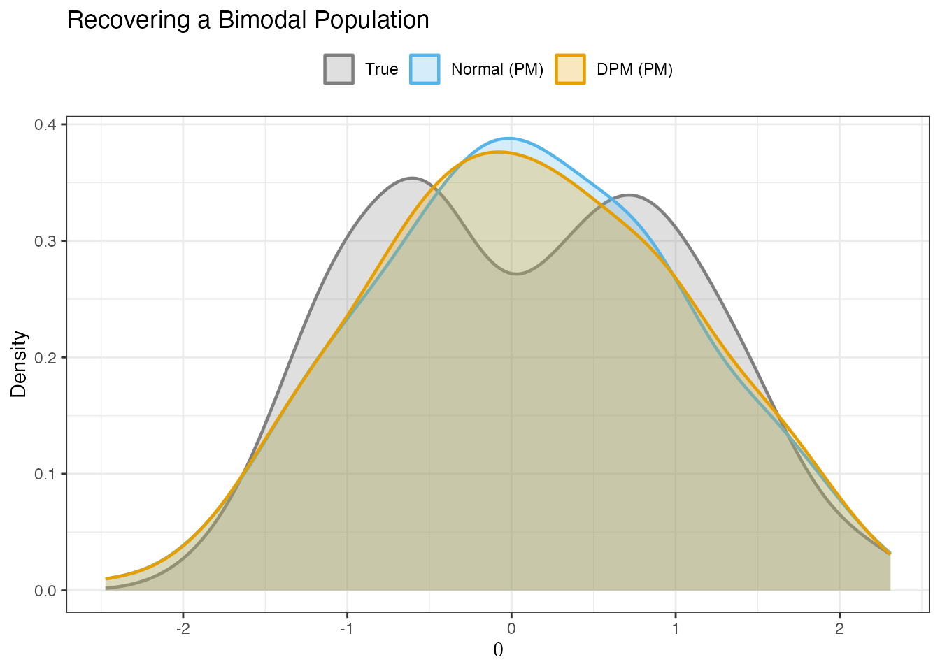

True bimodal density (gray) versus posterior mean densities under Normal (blue) and DPM (orange) priors. Posterior means are useful diagnostics but can understate distributional differences.

Take-away. When the true distribution departs from normality, the DPM prior supplies flexibility that the Normal prior cannot. WAIC may not detect this distinction because it evaluates item-response prediction, not ability-distribution recovery; posterior-mean densities are only a first diagnostic. For practical guidance on choosing the posterior summary that best serves your inferential goal, see Posterior Summaries.

Practical recommendation. For applied researchers who suspect non-normality, fit both priors and compare them using (1) WAIC for item-response prediction and (2) PM/CB/GR density plots for distributional recovery. In simulations where truth is known, use dpmirt_loss() to check whether the apparent distributional gain also improves the loss tied to your inferential goal.

6. Identification Strategies

Strategy	Rasch	2PL	3PL	How It Works
constrained_ability	Yes (Normal only)	Yes (Normal only)	Yes (Normal only)	Fix $\theta \sim N(0, 1)$ ; no hyperparameters
constrained_item	Yes (default)	Yes	No	Mean-center $\beta$ during MCMC (+ geom-mean $\lambda = 1$ for 2PL)
unconstrained	Yes	Yes (default)	Yes (default)	No constraints; post-hoc rescaling via dpmirt_rescale()

Compatibility rules. The unconstrained + post-hoc rescaling approach yields the most efficient MCMC sampler for DPM-IRT models. constrained_ability is incompatible with the DPM prior, and constrained_item is not implemented for 3PL. DPMirt raises an error for these combinations instead of silently changing the requested model.

# Rasch with unconstrained + post-hoc rescaling
fit <- dpmirt(data, model = "rasch", prior = "normal",
              identification = "unconstrained")

# 2PL with in-model constrained_item centering
fit <- dpmirt(data, model = "2pl", prior = "normal",
              identification = "constrained_item")

How to choose. For DPM models, use the defaults ("constrained_item" for Rasch, "unconstrained" for 2PL/3PL). For Normal-prior Rasch/2PL models, all three strategies are available. For Normal-prior 3PL, use "unconstrained" or "constrained_ability". The "constrained_ability" strategy gives the strongest $N(0,1)$ shrinkage.

7. Chain Continuation

When an initial run needs more iterations, dpmirt_resume() continues the sampler from its current state without recompilation.

# Initial fit
fit <- dpmirt(data, model = "rasch", prior = "dpm",
              niter = 5000, nburnin = 1000, seed = 42)

# Trace looks non-stationary...
plot(fit, type = "trace")

# Resume: add 10,000 more iterations (no burn-in needed)
resumed_samples <- dpmirt_resume(fit, niter_more = 10000)
resumed_fit <- dpmirt_rescale(resumed_samples)

With the step-by-step workflow:

samples <- dpmirt_sample(compiled, niter = 5000, nburnin = 1000)
resumed_samples <- dpmirt_resume(samples, niter_more = 10000)
resumed_fit <- dpmirt_rescale(resumed_samples)

dpmirt_resume() requires the compiled model’s C++ pointers to be alive in the same R session. Saved RDS fits and fixtures cannot restore those pointers; if they are expired or absent, recompile from the saved specification and start a new sampling run.

The returned dpmirt_samples object can then be passed through dpmirt_rescale() (which returns a dpmirt_fit) and dpmirt_estimates().

8. Model Comparison with WAIC

When available, each dpmirt_fit stores a WAIC (Watanabe–Akaike Information Criterion) value computed during sampling. The current implementation uses NIMBLE’s conditional online WAIC with its default data-node grouping; explicit person-level WAIC grouping is reserved for a later model-comparison upgrade. For chain-labeled multi-run fits, the top-level fit$waic is currently the mean of per-run WAIC values; dpmirt_diagnostics(fit)$waic_by_chain and dpmirt_diagnostics(fit)$waic_aggregation preserve that provenance. For single-run fits with finite comparable WAIC, lower values indicate better expected out-of-sample item-response prediction. For mean_of_chain_waic provenance, inspect waic_by_chain and waic_aggregation and interpret rankings cautiously rather than as pooled posterior WAIC.

comparison <- dpmirt_compare(fit_rasch_n, fit_rasch_dpm)
comparison

comparison <- dpmirt_compare(fit_rasch_n, fit_rasch_dpm)
knitr::kable(comparison, digits = 2, row.names = FALSE)

model	waic	delta_waic	waic_aggregation
RASCH-dpm	6078.17	0.00	single_chain
RASCH-normal	6079.03	0.86	single_chain

The delta_waic column shows the difference from the best model. You can compare any number of fits:

dpmirt_compare(fit_rasch_n, fit_rasch_dpm, fit_2pl)

Interpreting WAIC differences.

$|\Delta\text{WAIC}| < 2$ : Models essentially equivalent.

$2 < |\Delta\text{WAIC}| < 10$ : Moderate preference.

$|\Delta\text{WAIC}| > 10$ : Strong preference.

9. Data Formats

Matrix Format (Default)

Binary matrix with persons in rows and items in columns. Missing responses coded as NA.

head(sim$response[, 1:6])
#>      [,1] [,2] [,3] [,4] [,5] [,6]
#> [1,]    1    0    1    1    0    1
#> [2,]    0    1    0    1    1    0

Long Format

A data.frame with columns for person, item, and response. DPMirt detects the format automatically and converts internally.

head(response_long)
#>   person item response
#> 1      1    1        1
#> 2      1    2        0

fit <- dpmirt(response_long, model = "rasch", prior = "normal")

If the long-to-matrix conversion produces a very large or sparse matrix, verify dimensions with dpmirt_spec() before running the full pipeline.

10. Visualizations

DPMirt provides 12 plot types via plot(fit, type = ...). When ggplot2 is installed it is used automatically; otherwise base R graphics are produced.

Type	Description
density	Kernel density of posterior mean theta
items	Item parameter estimates with posterior intervals
trace	Log-likelihood trace (first-pass visual mixing check)
clusters	Active cluster count trace (DPM only)
dp_density	DP mixture density with credible band (DPM only; can be expensive)
icc	Item Characteristic Curves
wright_map	Wright map: items and persons on common logit scale
parameter_trace	Trace plots for individual parameters
caterpillar	Caterpillar plot of sorted estimates with CIs
density_compare	Overlaid densities from two fits
info	Test and item information functions (2PL/3PL)
pp_check	Posterior predictive check

plot(fit_rasch_dpm, type = "density")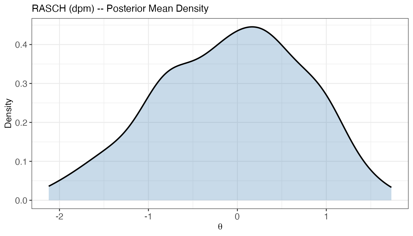

Posterior density of person abilities.

plot(fit_rasch_dpm, type = "items")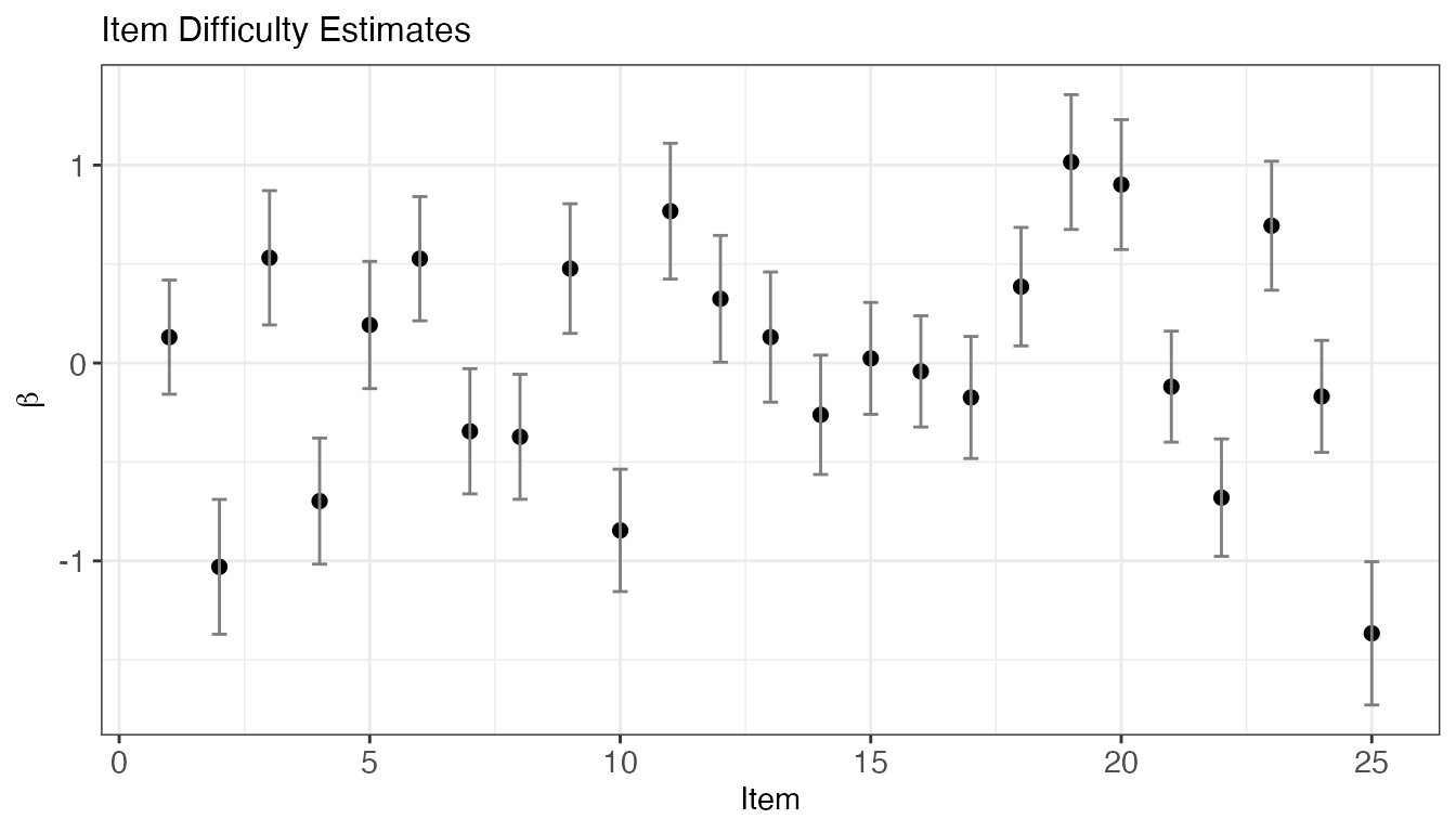

Item difficulty estimates with posterior intervals.

plot(fit_rasch_dpm, type = "trace")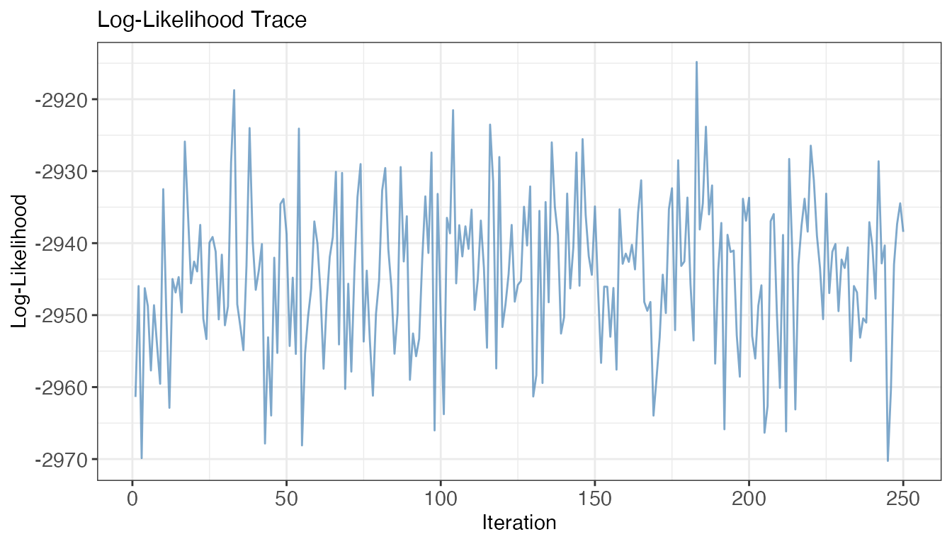

Log-likelihood trace.

plot(fit_rasch_dpm, type = "icc", items = 1:6)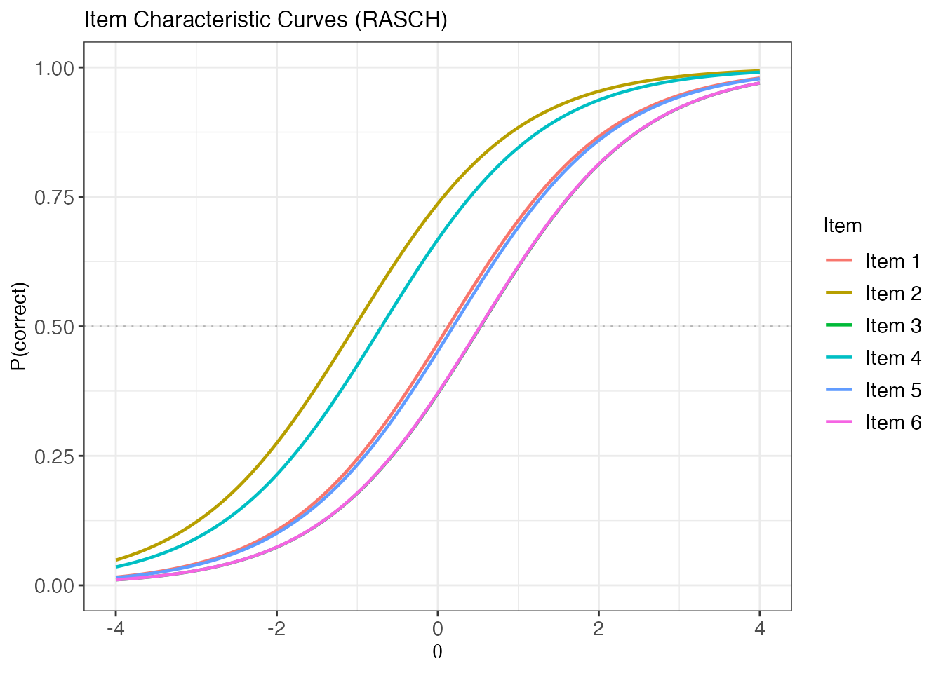

Item Characteristic Curves for items 1–6.

plot(fit_rasch_dpm, type = "wright_map")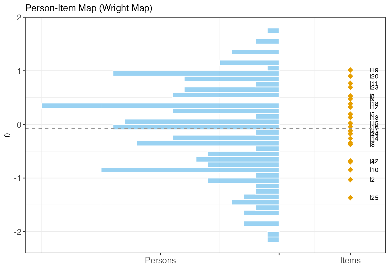

Wright map.

11. Summary and What’s Next?

This vignette covered the full model and workflow space in DPMirt:

Two workflow modes: one-step dpmirt() and the step-by-step pipeline for compile-once sampling while compiled objects are live.
Three IRT models: Rasch, 2PL, and 3PL, each with Normal or DPM priors.
Two parameterizations for 2PL/3PL: IRT and slope–intercept.
Three identification strategies with explicit compatibility limits: DPM rejects constrained_ability and 3PL rejects constrained_item.
Chain continuation with dpmirt_resume() when the compiled model pointer is still live.
Model comparison with WAIC via dpmirt_compare().
Twelve built-in plot types for posterior visualization.

Topic	Vignette	What
Choosing an estimator	Posterior Summaries	In-depth PM vs CB vs GR comparison; shrinkage diagnostics; loss evaluation
Setting DPM priors	Prior Elicitation	Optional DPprior calibration of alpha; Gamma(1, 3) fallback
NIMBLE internals	NIMBLE Internals	Custom sampler hooks, NIMBLE compilation model, advanced tuning

JoonHo Lee

2026-07-23