DPMirt: Bayesian Semiparametric Item Response Theory

Introduction

When using Item Response Theory models for educational and psychological assessment, researchers almost always assume that the latent traits—the abilities, proficiencies, or attitudes being measured—follow a normal distribution. This assumption is so deeply embedded in standard IRT software that it rarely receives explicit scrutiny. Yet the populations we study are often far from normal.

Consider students preparing for a high-stakes graduation exam: one group has mastered the curriculum, while another group is still struggling with foundational concepts. Or consider a clinical sample where most respondents fall in the typical range, but a meaningful minority exhibits extreme scores. In these settings, forcing a bell curve onto the latent trait distribution distorts individual ability estimates, misleads ranking decisions, and produces inaccurate pictures of the population.

DPMirt addresses this problem by replacing the parametric normal prior with a Dirichlet Process Mixture (DPM) prior on the latent trait distribution. The DPM prior is a Bayesian nonparametric tool that lets the data inform the shape of the ability distribution—whether it turns out to be unimodal, bimodal, skewed, or something else entirely—without requiring the researcher to choose a specific parametric form in advance. The package wraps the NIMBLE probabilistic programming engine and provides a complete workflow from data simulation through model fitting, posterior summarization, and diagnostics.

This vignette introduces the motivation, architecture, and model family of DPMirt, and provides a road map to the rest of the documentation.

Motivating Example: Why Normality Matters

The scenario

Imagine a curriculum-based mathematics assessment administered to a heterogeneous student population. Advanced-track students have had an additional year of instruction, while general-track students are still building fluency. The true ability distribution is genuinely bimodal—two overlapping groups with distinct centers.

We examine this scenario using pre-computed simulation results shipped with the package. The data were generated from a Rasch model with 25 items and 200 persons drawn from a bimodal ability distribution (a mixture of two normal components centered at $\theta = -1.5$ and $\theta = 1.5$ ). Two models were fit to these responses: one with a standard normal prior and one with a DPM prior.

sim <- readRDS(find_extdata("vignette_sim_bimodal.rds"))
fit_normal <- readRDS(find_extdata("vignette_fit_rasch_normal_bimodal.rds"))
fit_dpm <- readRDS(find_extdata("vignette_fit_rasch_dpm_bimodal.rds"))

The comparison

The figure below overlays three densities: the true generating distribution (gray), the posterior mean estimates from the normal-prior model (blue), and the posterior mean estimates from the DPM-prior model (orange).

if (requireNamespace("ggplot2", quietly = TRUE)) {
  library(ggplot2)

  true_theta <- sim$theta
  pm_normal  <- colMeans(fit_normal$theta_samp)
  pm_dpm     <- colMeans(fit_dpm$theta_samp)

  plot_df <- data.frame(
    value  = c(true_theta, pm_normal, pm_dpm),
    source = factor(rep(c("True", "Normal Prior (PM)", "DPM Prior (PM)"),
                        each = length(true_theta)),
                    levels = c("True", "Normal Prior (PM)", "DPM Prior (PM)"))
  )

  fill_vals  <- c("True" = unname(palette_dpmirt["true"]),
                   "Normal Prior (PM)" = unname(palette_dpmirt["normal"]),
                   "DPM Prior (PM)" = unname(palette_dpmirt["dpm"]))

  ggplot(plot_df, aes(x = value, fill = source, color = source)) +
    geom_density(alpha = 0.35, linewidth = 0.8) +
    scale_fill_manual(values = fill_vals) +
    scale_color_manual(values = fill_vals) +
    labs(x = expression(theta), y = "Density",
         title = "Normal vs. DPM Prior: Recovering a Bimodal Population",
         subtitle = "Rasch model, 25 items, 200 persons") +
    theme_minimal() +
    theme(legend.position = "bottom", legend.title = element_blank(),
          plot.title = element_text(face = "bold"))
}

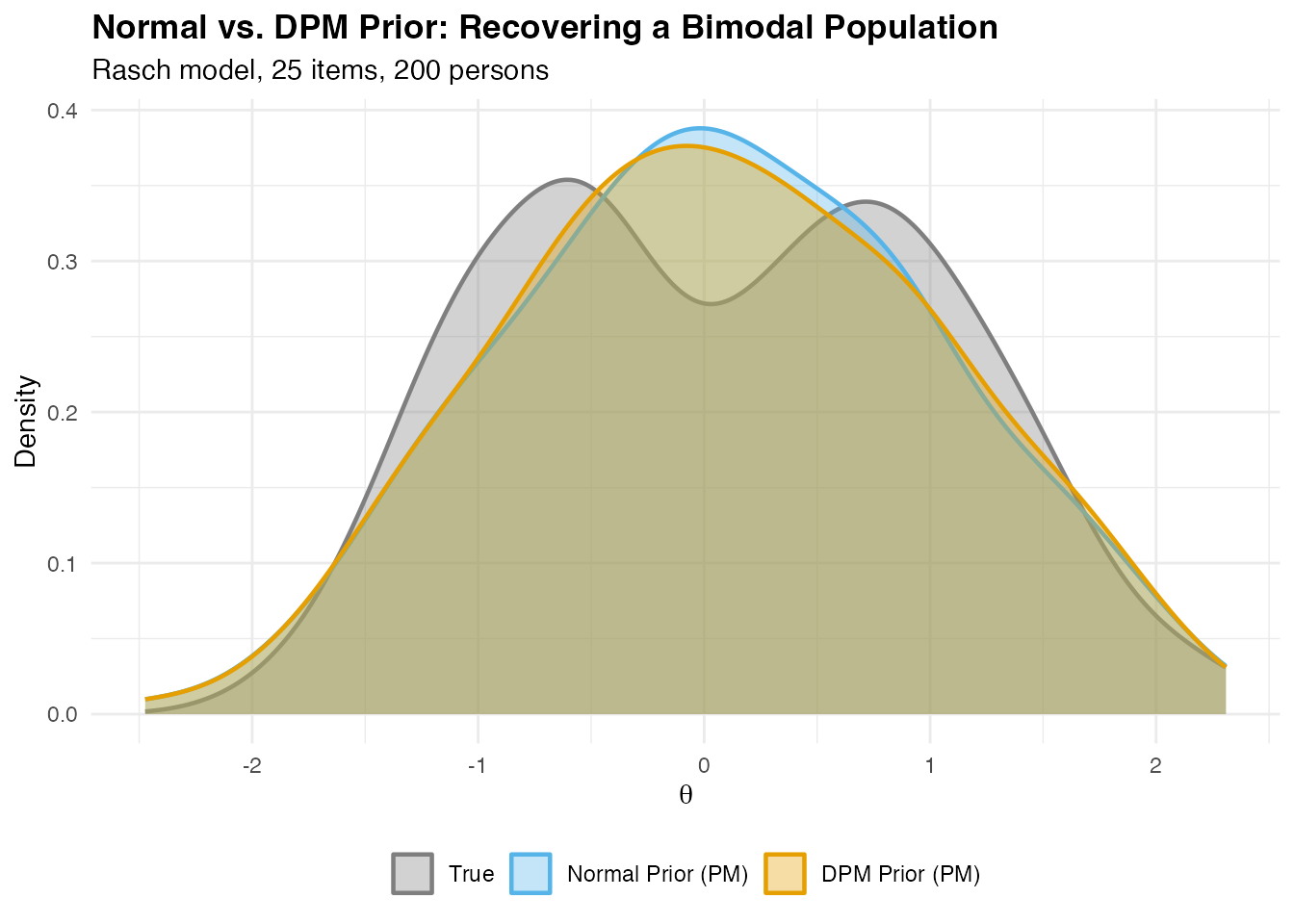
Recovered ability distributions under normal and DPM priors for a bimodal population. The normal prior shrinks estimates toward the center, masking the true bimodality. The DPM prior recovers the two-group structure.

What went wrong with the normal prior?

The normal-prior model has no mechanism to represent bimodality. Its posterior mean estimates are pulled toward a single central peak—a phenomenon called underdispersion or overshrinkage. The two modes of the true distribution collapse into one, and the tails are artificially thin.

Key insight. When the true ability distribution departs from normality, the normal-prior IRT model does not simply produce noisier estimates—it produces systematically biased estimates. High-ability students are pulled downward; low-ability students are pulled upward; and the entire empirical distribution function is distorted.

This has practical consequences. If a school district uses a cutoff to identify students for an enrichment program, the normal-prior estimates will undercount eligible students from the high-ability group. The DPM prior, by adapting to the data-generating shape, substantially reduces this bias.

What DPMirt Does

DPMirt provides a complete toolkit for Bayesian semiparametric IRT, organized into five functional layers:

arch_df <- data.frame(
  Layer = c("User Interface", "Step-by-Step",
            "Diagnostics & Visualization", "Simulation", "Integration"),
  Purpose = c("One-step fitting",
              "Fine-grained control over each pipeline stage",
              "MCMC assessment and result visualization",
              "Data generation and loss evaluation",
              "External package interoperability"),
  `Key Functions` = c(
    "dpmirt()",
    "dpmirt_spec(), dpmirt_compile(), dpmirt_sample(), dpmirt_rescale(), dpmirt_estimates()",
    "dpmirt_diagnostics(), plot(), dpmirt_plot_density(), dpmirt_plot_caterpillar()",
    "dpmirt_simulate(), dpmirt_loss()",
    "dpmirt_alpha_prior(), dpmirt_compare()"),
  check.names = FALSE
)
knitr::kable(arch_df, col.names = c("Layer", "Purpose", "Key Functions"),
             caption = "DPMirt package architecture")

DPMirt package architecture
Layer	Purpose	Key Functions
User Interface	One-step fitting	dpmirt()
Step-by-Step	Fine-grained control over each pipeline stage	dpmirt_spec(), dpmirt_compile(), dpmirt_sample(), dpmirt_rescale(), dpmirt_estimates()
Diagnostics & Visualization	MCMC assessment and result visualization	dpmirt_diagnostics(), plot(), dpmirt_plot_density(), dpmirt_plot_caterpillar()
Simulation	Data generation and loss evaluation	dpmirt_simulate(), dpmirt_loss()
Integration	External package interoperability	dpmirt_alpha_prior(), dpmirt_compare()

Most users will interact primarily with the User Interface layer. A single call to dpmirt() handles the entire pipeline—from building the NIMBLE model code, through compilation, MCMC sampling, post-hoc rescaling, and optional WAIC computation—returning a fitted model object ready for summarization and plotting. The fitted object also stores chain/run metadata (schema_version, chain_info, draw_index, and run_history) used by diagnostics and draw extraction. For users who need more control, the Step-by-Step layer exposes each stage as a separate function, following a compile-once, sample-many pattern while the compiled NIMBLE object is live in the current R session.

Three Inferential Goals

One of the central insights motivating DPMirt is that there is no single “best” point estimate of latent traits. Different applied questions demand different posterior summaries, and the choice of estimator should be driven by the inferential goal—not by convention.

Lee & Wind formalized three distinct goals for latent trait estimation:

goals_df <- data.frame(
  Goal = c("1. Individual traits", "2. Ranking", "3. Distribution"),
  Target = c("$\\theta_p$",
             "$R_p = \\text{rank}(\\theta_p)$",
             "$G_N(t) = N^{-1} \\sum I(\\theta_p \\le t)$"),
  Loss = c("MSEL", "MSELR", "ISE / KS"),
  Example = c("What is this student's ability?",
              "Which 5 students need intervention?",
              "What percentage exceed the cutoff?"),
  Estimator = c("Posterior Mean (PM)", "Triple-Goal (GR)",
                "Constrained Bayes (CB) / Triple-Goal (GR)")
)
knitr::kable(goals_df,
  col.names = c("Goal", "Target", "Loss Function",
                "Example Question", "Optimal Estimator"),
  caption = "Three inferential goals for latent trait estimation (Lee & Wind)",
  escape = FALSE)

Three inferential goals for latent trait estimation (Lee & Wind)
Goal	Target	Loss Function	Example Question	Optimal Estimator
1. Individual traits	$\theta_p$	MSEL	What is this student’s ability?	Posterior Mean (PM)
2. Ranking	$R_p = \text{rank}(\theta_p)$	MSELR	Which 5 students need intervention?	Triple-Goal (GR)
3. Distribution	$G_N(t) = N^{-1} \sum I(\theta_p \le t)$	ISE / KS	What percentage exceed the cutoff?	Constrained Bayes (CB) / Triple-Goal (GR)

Key insight. No single estimator simultaneously optimizes all three goals. The posterior mean (PM) minimizes individual mean squared error but produces an underdispersed empirical distribution, distorting rankings and distribution estimates. Constrained Bayes (CB) corrects the distribution but not the ranks. Only the triple-goal (GR) estimator of Shen and Louis (1998) simultaneously targets accurate ranking and distribution recovery.

DPMirt computes all three estimators from stored posterior samples, enabling researchers to choose the summary that matches their applied question. The benefit of using a DPM prior compounds with the right estimator choice: the DPM prior provides a more faithful posterior, from which the CB and GR estimators can extract more accurate summaries.

Model Family

DPMirt supports a complete family of unidimensional IRT models, crossing three item models with two latent trait priors:

model_df <- data.frame(
  Model = c("Rasch", "Rasch", "2PL", "2PL", "3PL", "3PL"),
  Prior = c("Normal", "DPM", "Normal", "DPM", "Normal", "DPM"),
  Parameters = c(
    "$\\beta_i$", "$\\beta_i$",
    "$\\beta_i, \\lambda_i$", "$\\beta_i, \\lambda_i$",
    "$\\beta_i, \\lambda_i, \\delta_i$",
    "$\\beta_i, \\lambda_i, \\delta_i$"),
  Parameterizations = c("IRT", "IRT", "IRT, SI", "IRT, SI",
                         "IRT, SI", "IRT, SI"),
  Identification = c(
    "Constrained item*, constrained ability, unconstrained",
    "Constrained item*, unconstrained",
    "Unconstrained*, constrained ability, constrained item",
    "Unconstrained*, constrained item",
    "Unconstrained*, constrained ability",
    "Unconstrained*")
)
knitr::kable(model_df,
  col.names = c("Model", "Prior", "Item Parameters",
                "Parameterizations", "Identification"),
  caption = "Supported model family (* = default identification strategy)",
  escape = FALSE)

Supported model family (* = default identification strategy)
Model	Prior	Item Parameters	Parameterizations	Identification
Rasch	Normal	$\beta_i$	IRT	Constrained item*, constrained ability, unconstrained
Rasch	DPM	$\beta_i$	IRT	Constrained item*, unconstrained
2PL	Normal	$\beta_i, \lambda_i$	IRT, SI	Unconstrained*, constrained ability, constrained item
2PL	DPM	$\beta_i, \lambda_i$	IRT, SI	Unconstrained*, constrained item
3PL	Normal	$\beta_i, \lambda_i, \delta_i$	IRT, SI	Unconstrained*, constrained ability
3PL	DPM	$\beta_i, \lambda_i, \delta_i$	IRT, SI	Unconstrained*

Parameterizations. The IRT form uses $\text{logit}(\pi_{ip}) = \lambda_i (\theta_p - \beta_i)$ ; the slope-intercept (SI) form uses $\text{logit}(\pi_{ip}) = \gamma_i + \lambda_i \theta_p$ . Both are available for 2PL and 3PL; the Rasch model uses IRT form only.
Identification. IRT models require constraints to resolve location (and, for 2PL/3PL, scale) indeterminacy. DPMirt supports constraining item parameters, constraining abilities, or leaving the model unconstrained with post-hoc rescaling. The unconstrained + rescaling approach is the default for 2PL/3PL, following Paganin et al. (2023). Some combinations are intentionally unavailable: DPM models reject constrained_ability, and 3PL models reject constrained_item.
DPM prior. Uses the Chinese Restaurant Process (CRP) representation with cluster atoms from a Normal-Inverse-Gamma base measure. The concentration parameter $\alpha$ receives a Gamma hyperprior—either the default $\text{Gamma}(1, 3)$ or an optional principled choice via DPprior.
3PL guessing. The 3PL model includes item-specific lower asymptote parameters $\delta_i$ . DPMirt reports posterior summaries and plots for $\delta$ where applicable. For simulation, reliability targeting is available through IRTsimrel for Rasch/2PL; 3PL currently uses DPMirt’s fallback generator and does not target target_rho.

Backbone References

DPMirt builds on three lines of methodological work, each credited here.

Paganin et al. (2023) established the computational framework: NIMBLE model code, custom MCMC samplers, post-hoc rescaling functions, and DP measure sampling routines. Their unconstrained + rescaling identification strategy and centered sampler for the SI parameterization form the backbone of DPMirt’s NIMBLE engine. The package wraps this validated codebase in a user-friendly API with programmatic model code generation.

Lee & Wind formalized the three inferential goals—individual trait estimation, ranking, and distribution recovery—and evaluated PM, CB, and GR estimators across the full Rasch/2PL/3PL model family under both parametric and semiparametric priors. A key finding was that test reliability is the dominant moderator: at high reliability, the combination of DPM prior with the GR estimator yields substantial gains for ranking and distribution recovery.

Lee (2026) developed the DPprior package for principled specification of the Gamma hyperprior on $\alpha$ . DPMirt can use this optional package when researchers express beliefs about expected latent subgroups and uncertainty; otherwise it falls back to the conservative $\text{Gamma}(1, 3)$ default. This is especially important when sample size is moderate and item quality is limited, where the prior on $\alpha$ can substantially influence posterior inference.

Installation

DPMirt requires NIMBLE as its MCMC backend. NIMBLE in turn requires a working C++ compiler (Rtools on Windows, Xcode Command Line Tools on macOS, or build-essential on Linux).

# From GitHub (development version)
# install.packages("remotes")
remotes::install_github("joonho112/DPMirt")

# Verify that NIMBLE is working
library(nimble)
nimbleOptions(verbose = FALSE)

We recommend also installing these optional packages:

# Visualization (highly recommended)
install.packages("ggplot2")

# Principled alpha elicitation
remotes::install_github("joonho112/DPprior")

# Reliability-targeted Rasch/2PL simulation
remotes::install_github("joonho112/IRTsimrel")

DPMirt works without the two optional GitHub packages above. Without DPprior, alpha-prior elicitation falls back to $\text{Gamma}(1, 3)$ . Without IRTsimrel, dpmirt_simulate() uses DPMirt’s internal fallback simulator, which does not target reliability.

After installation, load the package:

library(DPMirt)

Road Map to the Vignettes

DPMirt documentation is organized into two tracks. Applied researchers follow a progressive path from a quick first fit through the complete model workflow. Methodological researchers can dive into mathematical and computational details.

Applied Researchers Track

applied_df <- data.frame(
  Vignette = c("[Quick Start](quick-start.html)",
               "[Models and Workflow](models-and-workflow.html)",
               "[Posterior Summaries](posterior-summaries.html)",
               "[Prior Elicitation](prior-elicitation.html)",
               "[Simulation Study](simulation-study.html)"),
  Purpose = c("Your first IRT fit in 5 minutes",
              "Complete guide to all models and the step-by-step pipeline",
              "PM, CB, GR: when each estimator is optimal",
              "Principled DPM hyperprior selection via DPprior",
              "Replicating the evaluation framework from Lee & Wind"),
  Time = c("5 min", "30--40 min", "25--30 min", "20--25 min", "30--40 min")
)
knitr::kable(applied_df, col.names = c("Vignette", "Purpose", "Time"),
             caption = "Applied researchers track")

Applied researchers track
Vignette	Purpose	Time
Quick Start	Your first IRT fit in 5 minutes	5 min
Models and Workflow	Complete guide to all models and the step-by-step pipeline	30–40 min
Posterior Summaries	PM, CB, GR: when each estimator is optimal	25–30 min
Prior Elicitation	Principled DPM hyperprior selection via DPprior	20–25 min
Simulation Study	Replicating the evaluation framework from Lee & Wind	30–40 min

Recommended path for new users: Quick Start $\rightarrow$ Models and Workflow $\rightarrow$ Posterior Summaries. The Prior Elicitation and Simulation Study vignettes can be read in any order after that.

Methodological Researchers Track

methods_df <- data.frame(
  Vignette = c("[Mathematical Foundations](theory-irt-dpm.html)",
               "[NIMBLE Internals](nimble-internals.html)"),
  Purpose = c(
    "IRT model theory, DPM priors, identification, and posterior summary derivations",
    "Custom sampler hooks, compile-once pattern, and advanced NIMBLE configuration"),
  Time = c("45--60 min", "30--40 min")
)
knitr::kable(methods_df, col.names = c("Vignette", "Purpose", "Time"),
             caption = "Methodological researchers track")

Methodological researchers track
Vignette	Purpose	Time
Mathematical Foundations	IRT model theory, DPM priors, identification, and posterior summary derivations	45–60 min
NIMBLE Internals	Custom sampler hooks, compile-once pattern, and advanced NIMBLE configuration	30–40 min

Recommended path for methodologists: Start with Mathematical Foundations, then consult NIMBLE Internals. The Applied Track vignettes provide complementary hands-on demonstrations.

Reading paths by question

“I just want to fit a model quickly.” $\rightarrow$ Quick Start
“Should I use a normal or DPM prior?” $\rightarrow$ Models and Workflow, Section 2
“Which estimator should I report—PM, CB, or GR?” $\rightarrow$ Posterior Summaries
“How do I choose the concentration parameter alpha?” $\rightarrow$ Prior Elicitation
“I want to run a simulation study comparing priors.” $\rightarrow$ Simulation Study
“How does the DPM-IRT model work mathematically?” $\rightarrow$ Mathematical Foundations
“I need to customize the NIMBLE sampler configuration.” $\rightarrow$ NIMBLE Internals

References

Ghosh, M. (1992). Constrained Bayes estimation with applications. Journal of the American Statistical Association, 87(418), 533–540.

Lee, J. & Wind, S. Targeting toward inferential goals in Bayesian Rasch models for estimating person-specific latent traits. OSF Preprint. https://doi.org/10.31219/osf.io/qrw4n

Lee, J. (2026). Design-conditional prior elicitation for Dirichlet Process mixtures: A unified framework for cluster counts and weight control. arXiv preprint arXiv:2602.06301. https://arxiv.org/abs/2602.06301

Paganin, S., Paciorek, C. J., Wehrhahn, C., Rodríguez, A., Rabe-Hesketh, S., & de Valpine, P. (2023). Computational strategies and estimation performance with Bayesian semiparametric item response theory models. Journal of Educational and Behavioral Statistics, 48(2), 147–188. https://doi.org/10.3102/10769986221136105

Shen, W., & Louis, T. A. (1998). Triple-goal estimates in two-stage hierarchical models. Journal of the Royal Statistical Society: Series B, 60(2), 455–471.

For questions, bug reports, or feature requests, please visit the GitHub repository.

JoonHo Lee

2026-07-23