Principled Prior Elicitation for the DP Concentration Parameter
JoonHo Lee
2026-07-23
Source:vignettes/prior-elicitation.Rmd
prior-elicitation.RmdOverview
Every Dirichlet Process Mixture (DPM) model contains a concentration parameter that controls how much the nonparametric prior deviates from a single parametric component. Choosing well is not just a technical detail — it shapes cluster formation, posterior shrinkage, and the balance between flexibility and parsimony.
This vignette covers:
- Why matters — its three operational dimensions.
- Paganin default vs. principled elicitation — when is adequate and when it is not.
- DPprior integration — several routes to set in DPMirt.
- Two strategies from Lee (2026) — DP-diffuse and DP-inform.
- Sensitivity analysis — comparing posteriors under different priors.
- Fallback behavior — what happens when DPprior is not installed.
- Custom base measure tuning — advanced hyperparameter control.
Why Alpha Matters
The concentration parameter operates along three dimensions that jointly determine the behavior of the DP prior.
Dimension 1: Number of Clusters
The expected number of distinct clusters among observations is approximately
Larger implies more clusters; smaller concentrates the posterior onto fewer groups.
Dimension 2: Weight Concentration
The first stick-breaking weight follows . When is small, is large and most mass is captured by a single component. When is large, mass spreads across many components.
Dimension 3: Posterior Shrinkage
In IRT, the prior on acts as a regularizer. A DPM prior with small shrinks person abilities toward fewer cluster centers, closely resembling a parametric Normal prior. A DPM prior with large allows each person to retain more of their data-driven estimate, reducing shrinkage at the cost of higher variance.
Key insight: The choice of is not merely a tuning knob — it encodes a substantive belief about the heterogeneity of the latent trait distribution. Getting it wrong can either mask genuine subgroups (too small) or fragment a homogeneous population (too large).
Paganin Default vs. Principled Elicitation
Paganin et al. (2023) use as a default. This prior has mean and is concentrated near zero, strongly favoring few clusters.
For many educational testing applications where the latent trait is approximately unimodal, this default is reasonable. However, it can be overly restrictive when: - The population is known to be heterogeneous (e.g., mixed clinical groups). - Sample size is large () and the data can support many clusters. - The research question specifically concerns subgroup detection.
Lee (2026) provides a principled alternative through the DPprior package, which uses Two-Stage Moment Matching (TSMM) to translate a researcher’s belief about the expected number of clusters into a calibrated hyperprior. The updated DPprior package also provides diagnostic tools for assessing dominance risk and prior quality, as well as a dual-anchor calibration framework for weight-constrained elicitation.
alpha_grid <- seq(0, 5, length.out = 500)
dens_default <- dgamma(alpha_grid, shape = 1, rate = 3)

plot(alpha_grid, dens_default, type = "l", lwd = 2, col = pal$reference,
     xlab = expression(alpha), ylab = "Density",
     main = expression(paste("Paganin default: ", alpha, " ~ Gamma(1, 3)")))
abline(v = 1/3, lty = 2, col = pal$reference)
text(1.2, max(dens_default) * 0.8,
bquote(E[alpha] == .(round(1/3, 2))), col = pal$reference)![The Paganin default Gamma(1, 3) prior for alpha, with implied E[alpha] = 0.33.](prior-elicitation_files/figure-html/paganin-default-1.png)
The Paganin default Gamma(1, 3) prior for alpha, with implied E[alpha] = 0.33.
DPprior Integration
DPMirt offers several ways to set the prior, ranging from the conservative default to fully manual DPprior workflows. DPprior is optional: when it is unavailable, DPMirt falls back to .
Method 1: dpmirt_alpha_prior() Wrapper
The simplest approach is the standalone elicitation function, which
returns a named vector c(a = ..., b = ...):
# Expect ~5 clusters among 200 persons, medium confidence
ab <- dpmirt_alpha_prior(N = 200, mu_K = 5, confidence = "medium")
#> Alpha prior: Gamma(1.85, 2.21) [E[alpha]=0.84]
ab
#>        a        b
#> 1.848904 2.212652Method 2: One-Step Auto-Elicitation
In the one-step wrapper, set mu_K and optionally
confidence to ask DPMirt to elicit the prior before model
construction:
fit <- dpmirt(
  data,
  model      = "rasch",
  prior      = "dpm",
  mu_K       = 5,
  confidence = "medium",
  niter      = 10000,
  nburnin    = 2000
)
This path calls dpmirt_alpha_prior() only when
prior = "dpm", alpha_prior = NULL, and
mu_K is not NULL. If mu_K = NULL,
the one-step wrapper uses the conservative
default.
Method 3: Elicit Then Pass to dpmirt()
Elicit the prior first with dpmirt_alpha_prior(), then
pass the result directly as alpha_prior:
ab <- dpmirt_alpha_prior(N = 200, mu_K = 5, confidence = "medium")

fit <- dpmirt(
  data,
  model       = "rasch",
  prior       = "dpm",
  alpha_prior = ab,
  niter       = 10000,
  nburnin     = 2000
)
Method 4: Manual DPprior Workflow
For maximum control, call DPprior directly and pass the result:
library(DPprior)

fit_prior <- DPprior_fit(J = 200, mu_K = 5, confidence = "medium")
#> Warning: HIGH DOMINANCE RISK: P(w1 > 0.5) = 60.4% exceeds 40%.
#>   This may indicate unintended prior behavior (Lee, 2026).
#>   Consider using DPprior_dual() for weight-constrained elicitation.
#>   See ?DPprior_diagnostics for interpretation.
print(fit_prior)
#> DPprior Prior Elicitation Result
#> =============================================
#>
#> Gamma Hyperprior: α ~ Gamma(a = 1.8489, b = 2.2127)
#>   E[α] = 0.836, SD[α] = 0.615
#>
#> Target (J = 200):
#>   E[K_J]   = 5.00
#>   Var(K_J) = 10.00
#>   (from confidence = 'medium')
#>
#> Achieved:
#>   E[K_J] = 5.000000, Var(K_J) = 10.000000
#>   Residual = 6.79e-11
#>
#> Method: A2-MN (6 iterations)
#>
#> Dominance Risk: HIGH ✘ (P(w₁>0.5) = 60%)
# Pass the DPprior_fit object to dpmirt
fit <- dpmirt(
  data,
  model       = "rasch",
  prior       = "dpm",
  alpha_prior = fit_prior,
  niter       = 10000
)
Method 5: Return the Full DPprior_fit Object
For access to diagnostics and convergence information, use
return_fit = TRUE:
# Get the full DPprior_fit object
fit_prior <- dpmirt_alpha_prior(N = 200, mu_K = 5, confidence = "medium",
                                 return_fit = TRUE)
#> Alpha prior: Gamma(1.85, 2.21) [E[alpha]=0.84]

# Inspect the result
print(fit_prior)
#> DPprior Prior Elicitation Result
#> =============================================
#>
#> Gamma Hyperprior: α ~ Gamma(a = 1.8489, b = 2.2127)
#>   E[α] = 0.836, SD[α] = 0.615
#>
#> Target (J = 200):
#>   E[K_J]   = 5.00
#>   Var(K_J) = 10.00
#>   (from confidence = 'medium')
#>
#> Achieved:
#>   E[K_J] = 5.000000, Var(K_J) = 10.000000
#>   Residual = 6.79e-11
#>
#> Method: A2-MN (6 iterations)
#>
#> Dominance Risk: HIGH ✘ (P(w₁>0.5) = 60%)

# Pass directly to dpmirt (DPprior_fit objects are accepted)
# fit <- dpmirt(data, prior = "dpm", alpha_prior = fit_prior)
Confidence Levels
The confidence argument controls how tightly the prior
concentrates around the expected cluster count. It maps to the variance
of the implied prior on
:
conf_levels <- c("low", "medium", "high")
conf_results <- lapply(conf_levels, function(cl) {
  fp <- DPprior_fit(J = 200, mu_K = 5, confidence = cl)
  data.frame(
    Confidence = cl,
    a          = round(fp$a, 3),
    b          = round(fp$b, 3),
    E_alpha    = round(fp$a / fp$b, 3),
    CV_alpha   = round(1 / sqrt(fp$a), 3),
    Var_K      = round(fp$target$var_K, 2),
    stringsAsFactors = FALSE
  )
})
#> Warning: HIGH DOMINANCE RISK: P(w1 > 0.5) = 64.3% exceeds 40%.
#>   This may indicate unintended prior behavior (Lee, 2026).
#>   Consider using DPprior_dual() for weight-constrained elicitation.
#>   See ?DPprior_diagnostics for interpretation.
#> Warning: HIGH DOMINANCE RISK: P(w1 > 0.5) = 60.4% exceeds 40%.
#>   This may indicate unintended prior behavior (Lee, 2026).
#>   Consider using DPprior_dual() for weight-constrained elicitation.
#>   See ?DPprior_diagnostics for interpretation.
#> Warning: HIGH DOMINANCE RISK: P(w1 > 0.5) = 58.7% exceeds 40%.
#>   This may indicate unintended prior behavior (Lee, 2026).
#>   Consider using DPprior_dual() for weight-constrained elicitation.
#>   See ?DPprior_diagnostics for interpretation.
conf_table <- do.call(rbind, conf_results)
knitr::kable(conf_table,
             caption = "Confidence levels and their implied hyperparameters (N = 200, mu_K = 5).",
align = "lccccc")| Confidence | a | b | E_alpha | CV_alpha | Var_K |
|---|---|---|---|---|---|
| low | 0.695 | 0.779 | 0.892 | 1.200 | 20 |
| medium | 1.849 | 2.213 | 0.836 | 0.735 | 10 |
| high | 4.944 | 6.087 | 0.812 | 0.450 | 6 |
Interpretation: Higher confidence concentrates the Gamma prior (lower CV), constraining and thereby the cluster count. Low confidence yields a diffuse prior that lets the data determine cluster structure. The confidence levels target the same expected cluster count, but the fitted Gamma mean for can shift slightly; the main effect is reduced prior dispersion around the cluster-count target.
Note that DPprior calls are analytic (closed-form or fast Newton iteration) and complete in milliseconds — no MCMC is involved.
Two Strategies from Lee (2026)
The APM manuscript (Lee & Wind) identifies two complementary approaches to specifying :
DP-Diffuse (Exploratory)
Use when you have little domain knowledge about population heterogeneity. The goal is a prior that is minimally informative yet properly calibrated to the sample size:
# DP-diffuse: set mu_K to log(N), low confidence
N <- 200
mu_K_diffuse <- max(3, ceiling(log(N)))  # 6 for N = 200

ab_diffuse <- dpmirt_alpha_prior(N = N, mu_K = mu_K_diffuse,
                                  confidence = "low")
#> Alpha prior: Gamma(0.84, 0.74) [E[alpha]=1.14]
cat("DP-diffuse: Gamma(", round(ab_diffuse["a"], 2), ", ",
    round(ab_diffuse["b"], 2), ")\n", sep = "")
#> DP-diffuse: Gamma(0.84, 0.74)
cat("  E[alpha] =", round(ab_diffuse["a"] / ab_diffuse["b"], 2), "\n")
#>   E[alpha] = 1.14
This shares the default cluster-count target
mu_K = max(3, ceiling(log(N))) used by
dpmirt_alpha_prior(N), but the explicit
confidence = "low" choice is deliberately more diffuse than
the function’s default confidence = "medium". The one-step
dpmirt() wrapper does not auto-elicit unless you set
mu_K; with mu_K = NULL and
alpha_prior = NULL, it uses the conservative
default.
DP-Inform (Domain-Driven)
Use when substantive knowledge suggests a specific number of latent subgroups. For example, an assessment designed to distinguish remedial, proficient, and advanced learners might target :
# DP-inform: domain-driven belief of 3 subgroups, high confidence
ab_inform <- dpmirt_alpha_prior(N = 200, mu_K = 3, confidence = "high")
#> Alpha prior: Gamma(2.88, 7.61) [E[alpha]=0.38]
cat("DP-inform: Gamma(", round(ab_inform["a"], 2), ", ",
    round(ab_inform["b"], 2), ")\n", sep = "")
#> DP-inform: Gamma(2.88, 7.61)
cat("  E[alpha] =", round(ab_inform["a"] / ab_inform["b"], 2), "\n")
#>   E[alpha] = 0.38
Visual Comparison
alpha_grid <- seq(0.01, 8, length.out = 500)

dens_diffuse <- dgamma(alpha_grid, shape = ab_diffuse["a"],
                        rate = ab_diffuse["b"])
dens_inform  <- dgamma(alpha_grid, shape = ab_inform["a"],
                        rate = ab_inform["b"])
dens_paganin <- dgamma(alpha_grid, shape = 1, rate = 3)

plot(alpha_grid, dens_diffuse, type = "l", lwd = 2, col = pal$semiparametric,
     xlab = expression(alpha), ylab = "Density",
     ylim = c(0, max(c(dens_diffuse, dens_inform, dens_paganin)) * 1.1),
     main = "Alpha prior comparison")
lines(alpha_grid, dens_inform, lwd = 2, col = pal$parametric)
lines(alpha_grid, dens_paganin, lwd = 2, col = pal$reference, lty = 2)
legend("topright",
       legend = c(paste0("DP-diffuse (low, mu_K=", mu_K_diffuse, ")"),
                   "DP-inform (high, mu_K=3)",
                   "Paganin Gamma(1,3)"),
       col    = c(pal$semiparametric, pal$parametric, pal$reference),
       lwd    = 2, lty = c(1, 1, 2), bty = "n")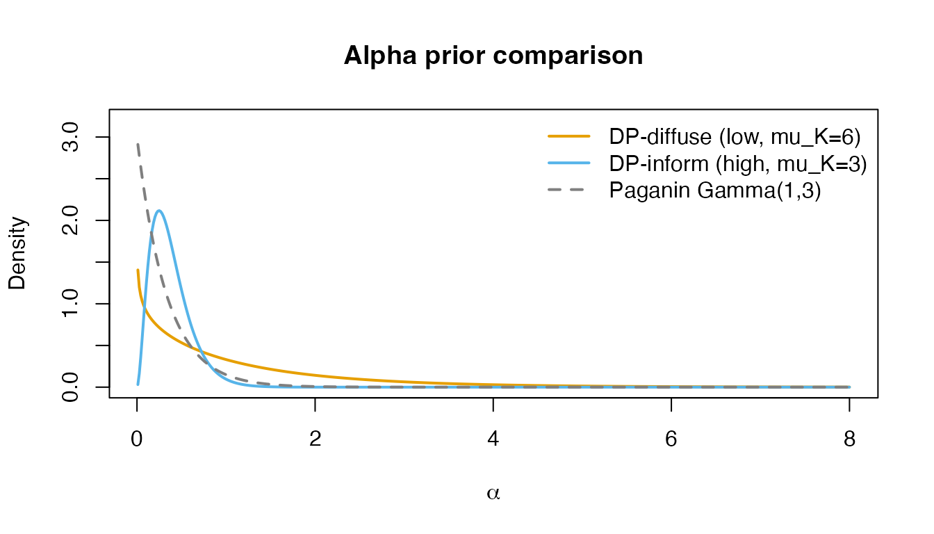
Comparing DP-diffuse and DP-inform alpha priors.
Sensitivity Analysis
A responsible Bayesian analysis examines how conclusions change under different prior specifications. Here we compare posterior results from three priors applied to the same data.
The compact fixtures below retain evenly thinned posterior draws from pre-computed Rasch-DPM fits on the same bimodal data set (, ):
sens <- readRDS(find_extdata("vignette_sensitivity_fits.rds"))

prior_labels <- c(
  default = "Paganin Gamma(1,3)",
  broad   = "Broad Gamma(0.5,1)",
  inform  = "Informative Gamma(3,1)"
)

# sens contains:
#   $default   - Gamma(1, 3) [Paganin default]
#   $broad     - Gamma(0.5, 1) [manual broad prior]
#   $inform    - Gamma(3, 1) [manual informative prior]
Posterior Density Comparison
# Extract posterior mean theta for each fit
est_paganin <- dpmirt_estimates(sens$default, methods = "pm")
est_diffuse <- dpmirt_estimates(sens$broad, methods = "pm")
est_inform  <- dpmirt_estimates(sens$inform,  methods = "pm")

dens_p <- density(est_paganin$theta$theta_pm)
dens_d <- density(est_diffuse$theta$theta_pm)
dens_i <- density(est_inform$theta$theta_pm)

xlim <- range(c(dens_p$x, dens_d$x, dens_i$x))
ylim <- c(0, max(c(dens_p$y, dens_d$y, dens_i$y)) * 1.1)

plot(dens_p, xlim = xlim, ylim = ylim, col = pal$reference, lwd = 2,
     lty = 2, main = "Posterior theta density under different alpha priors",
     xlab = expression(theta), ylab = "Density")
lines(dens_d, col = pal$semiparametric, lwd = 2)
lines(dens_i, col = pal$parametric, lwd = 2)
legend("topright",
       legend = unname(prior_labels[c("default", "broad", "inform")]),
       col = c(pal$reference, pal$semiparametric, pal$parametric),
       lwd = 2, lty = c(2, 1, 1), bty = "n")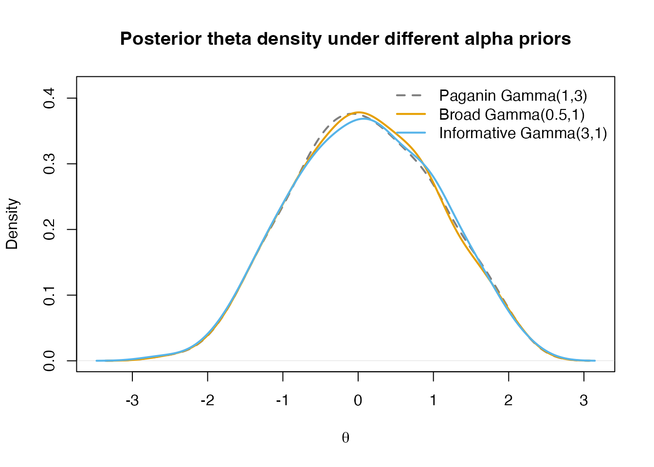
Posterior mean theta densities under three alpha priors. When the data are informative, the posteriors converge despite different priors.
Cluster Count Comparison
cluster_summary <- data.frame(
  Prior          = unname(prior_labels[c("default", "broad", "inform")]),
  Median_K       = c(median(sens$default$cluster_info$n_clusters),
                     median(sens$broad$cluster_info$n_clusters),
                     median(sens$inform$cluster_info$n_clusters)),
  Mean_K         = c(mean(sens$default$cluster_info$n_clusters),
                     mean(sens$broad$cluster_info$n_clusters),
                     mean(sens$inform$cluster_info$n_clusters)),
  Posterior_alpha = c(
    mean(sens$default$other_samp[, "alpha"]),
    mean(sens$broad$other_samp[, "alpha"]),
    mean(sens$inform$other_samp[, "alpha"])
  ),
  WAIC           = c(sens$default$waic,
                     sens$broad$waic,
                     sens$inform$waic)
)
cluster_summary$Median_K <- round(cluster_summary$Median_K, 1)
cluster_summary$Mean_K   <- round(cluster_summary$Mean_K, 1)
cluster_summary$Posterior_alpha <- round(cluster_summary$Posterior_alpha, 3)
cluster_summary$WAIC     <- round(cluster_summary$WAIC, 1)

knitr::kable(cluster_summary,
             caption = "Sensitivity analysis: cluster counts and WAIC under three alpha priors.",
align = "lcccc")| Prior | Median_K | Mean_K | Posterior_alpha | WAIC |
|---|---|---|---|---|
| Paganin Gamma(1,3) | 3 | 3.1 | 0.388 | 4010.5 |
| Broad Gamma(0.5,1) | 2 | 3.0 | 0.482 | 4009.8 |
| Informative Gamma(3,1) | 10 | 9.9 | 2.395 | 4011.5 |
Takeaway: When data are moderately informative (say, and ), the posterior distributions of theta tend to be robust to the choice of alpha prior. The main differences appear in the number of active clusters and the posterior uncertainty around alpha itself. WAIC can help assess item-response prediction, but differences are often small and do not by themselves establish ability-distribution recovery.
The convergence observed here reflects the moderately high reliability () of the 25-item test. For shorter tests with lower reliability (), the alpha prior may exert stronger influence on the posterior because the data provide less information to overcome the prior. See Posterior Summaries for a detailed analysis of how reliability moderates both estimator choice and prior choice.
Fallback Behavior
When the DPprior package is not installed, DPMirt falls back gracefully to the Paganin default with an informative message:
# Simulate what happens without DPprior
# (dpmirt_alpha_prior handles this internally)
if (!has_dpprior) {
  ab_fallback <- dpmirt_alpha_prior(N = 200)
  cat("Returned:", ab_fallback, "\n")
} else {
  cat("With DPprior installed, the package uses principled elicitation.\n")
  cat("Without DPprior, it returns c(a = 1, b = 3) with a message:\n\n")
  cat('  "DPprior not installed. Using default: Gamma(1, 3)\n')
  cat('   [Paganin et al., 2023].\n')
  cat('   Install DPprior for principled alpha elicitation:\n')
  cat('   remotes::install_github(\\"joonho112/DPprior\\")"\n')
}
#> With DPprior installed, the package uses principled elicitation.
#> Without DPprior, it returns c(a = 1, b = 3) with a message:
#>
#>   "DPprior not installed. Using default: Gamma(1, 3)
#>    [Paganin et al., 2023].
#>    Install DPprior for principled alpha elicitation:
#>    remotes::install_github(\"joonho112/DPprior\")"
This design ensures that DPMirt works out of the box. Installing
DPprior enables calibrated alternatives when you have a target expected
cluster count or want to inspect the full DPprior fit. DPprior is listed
in Suggests, not Imports, so it is never a
hard dependency.
Advanced: Custom Base Measure
The DP base measure determines the shape of each mixture component. DPMirt uses a Normal–Inverse-Gamma base:
The Paganin defaults are , , . These yield wide cluster means and diffuse cluster variances, appropriate for standardized IRT scales.
To customize:
# Wider cluster means, more concentrated cluster variances
fit <- dpmirt(
  data,
  model        = "rasch",
  prior        = "dpm",
  mu_K         = 5,
  confidence   = "medium",
  base_measure = list(s2_mu = 3, nu1 = 2.01, nu2 = 1.01),
  niter        = 10000
)
The step-by-step interface gives direct access:
spec <- dpmirt_spec(
  data,
  model        = "rasch",
  prior        = "dpm",
  alpha_prior  = c(a = 1, b = 3),
  base_measure = list(s2_mu = 3, nu1 = 2.01, nu2 = 1.01)
)

# Inspect what was set
spec$constants$s2_mu   # 3
spec$constants$nu1     # 2.01
spec$constants$nu2     # 1.01
Base Measure Hyperparameter Effects
| Hyperparameter | Default | Effect of Increasing |
|---|---|---|
| 2 | Wider spread of cluster means — clusters can be further apart | |
| 2.01 | Tighter cluster variances (more concentrated components) | |
| 1.01 | Wider cluster variances (more diffuse components) |
Practical guidance: For most IRT applications, the Paganin defaults work well. Increase if you expect latent subgroups separated by more than 3–4 standard deviations (e.g., combined clinical and non-clinical samples).
Elicitation Decision Flowchart
The following summary may help decide which approach to use:
| Scenario | Recommended approach | Code |
|---|---|---|
| Conservative default | Paganin Gamma(1,3) | dpmirt(data, prior = "dpm") |
| No domain knowledge, exploratory | DP-diffuse | dpmirt(data, prior = "dpm", mu_K = max(3, ceiling(log(N))), confidence = "low") |
| Substantive belief about subgroups | DP-inform | dpmirt(data, prior = "dpm", mu_K = 3, confidence = "high") |
| Reproducing Paganin et al. | Manual Gamma(1,3) | dpmirt(data, prior = "dpm", alpha_prior = c(1, 3)) |
| Comparing priors | Sensitivity analysis | Fit multiple models, compare posterior summaries and predictive WAIC |
| DPprior not available | Automatic fallback |
dpmirt(data, prior = "dpm", mu_K = 5) —
falls back to Gamma(1,3) with message |
What’s Next?
Now that you can set principled priors for , the following vignettes show how to put them to work:
| Vignette | Why read it |
|---|---|
| Quick Start | End-to-end pipeline with data simulation, fitting, and estimation |
| Simulation Study | Full factorial study comparing Normal vs. DPM priors under different conditions |
| NIMBLE Internals | How DPMirt generates NIMBLE code, compiles, and samples |
References
Lee, J. (2026). Design-conditional prior elicitation for Dirichlet Process mixtures: A unified framework for cluster counts and weight control. arXiv preprint arXiv:2602.06301. https://arxiv.org/abs/2602.06301
Lee, J. & Wind, S. Targeting toward inferential goals in Bayesian Rasch models for estimating person-specific latent traits. OSF Preprint. https://doi.org/10.31219/osf.io/qrw4n
Paganin, S., Paciorek, C. J., Wehrhahn, C., Rodríguez, A., Rabe-Hesketh, S., & de Valpine, P. (2023). Computational strategies and estimation performance with Bayesian semiparametric item response theory models. Journal of Educational and Behavioral Statistics, 48(2), 147–188. https://doi.org/10.3102/10769986221136105