svyder: Design Effect Ratio Diagnostics for Bayesian Survey Models • svyder

Design Effect Ratio diagnostics for Bayesian survey models — which parameters actually need a survey-design correction, and which are better left alone?

The problem

When you fit a Bayesian hierarchical model to complex survey data — a weighted pseudo-posterior — the posterior does not automatically reflect the sampling design. The usual repair is to rescale the whole posterior toward a design-based sandwich variance. Applied to every parameter that is a mistake: a within-group covariate genuinely needs its interval widened, but a shrinkage-protected random effect or a between-group coefficient gets its already-narrow interval crushed.

svyder computes a per-parameter Design Effect Ratio (DER) — the ratio of a parameter’s design-based sandwich variance to its model posterior variance — and uses it to correct only the parameters that need it.

DER > 1 — the posterior understates design uncertainty → widen it.
DER ≈ 1 — already calibrated → leave it alone.
DER < 1 — the posterior is already wider than the target → correcting would wrongly narrow it and destroy the shrinkage protection.

When should I use svyder?

You fit a Bayesian hierarchical / multilevel model to data from a complex survey (unequal weights, clustering, stratification).
You want to know which coefficients and random effects are sensitive to the design — not just a single global design effect.
You want a defensible, selective correction rather than a blanket rescaling of the whole posterior.

Installation

# install.packages("pak")
pak::pak("joonho112/svyder")

Quick start (5 minutes, no Stan required)

svyder ships two datasets with pre-computed posterior draws, so you can run the whole pipeline immediately.

library(svyder)
data(nsece_demo)   # synthetic, NSECE-like survey data: 6,785 units, 51 states, 644 PSUs

result <- der_diagnose(
  nsece_demo$draws,
  y = nsece_demo$y, X = nsece_demo$X,
  group   = nsece_demo$group,
  weights = nsece_demo$weights,
  cluster = nsece_demo$psu,          # the design PSU  ->  a *design-based* target
  family  = "binomial",
  sigma_theta = nsece_demo$sigma_theta,
  param_types = nsece_demo$param_types,
  verbose = FALSE
)
result
#> svyder diagnostic (54 parameters)
#>   Family: binomial | N = 6785 | J = 51
#>   Target: 644 cluster(s) | meat: centered, DF-corrected | weights: unit_mean
#>   DER range: [0.235, 5.308]
#>   Tier III (DER undefined): sigma_theta
#>   Threshold (tau): 1.20
#>   Flagged: 30 / 54 (55.6%)
#> 
#>   Flagged parameters:
#>     beta[2]              DER = 2.689  [I-a] -> CORRECT
#>     theta[1]             DER = 3.386  [II] -> CORRECT
#>     theta[4]             DER = 2.210  [II] -> CORRECT
#>     theta[5]             DER = 1.568  [II] -> CORRECT
#>     theta[6]             DER = 2.104  [II] -> CORRECT
#>     theta[7]             DER = 2.232  [II] -> CORRECT
#>     theta[9]             DER = 5.308  [II] -> CORRECT
#>     theta[11]            DER = 2.655  [II] -> CORRECT
#>     theta[15]            DER = 1.576  [II] -> CORRECT
#>     theta[18]            DER = 4.025  [II] -> CORRECT
#>     ... and 20 more
#> 
#>   Correction applied: 30 parameter(s) rescaled
#>   Compute time: 0.023 sec

der_diagnose() runs the three-step compute → classify → correct pipeline in one call.

Which parameters were flagged?

head(tidy(result), 3)   # the three fixed effects
#>            term   estimate  std.error       der tier  action flagged
#> beta[1] beta[1]  0.2498445 0.14735061 0.2626885  I-b  retain   FALSE
#> beta[2] beta[2] -0.1494408 0.02604573 2.6894416  I-a CORRECT    TRUE
#> beta[3] beta[3]  0.1610078 0.20239837 0.3430527  I-b  retain   FALSE
#>         scale_factor
#> beta[1]     1.000000
#> beta[2]     1.639952
#> beta[3]     1.000000

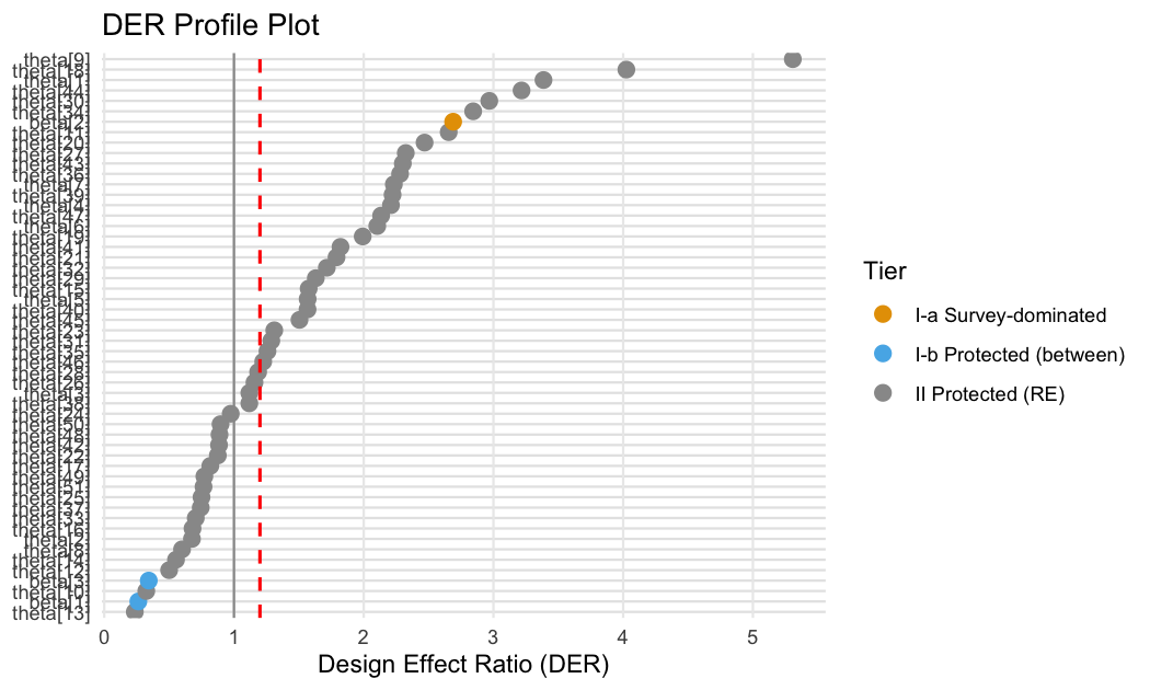
The within-state poverty coefficient (beta[2]) is flagged — Tier I-a, DER ≈ 2.7 — and its posterior is widened. The two between-state coefficients sit well below the threshold and are left untouched (Tier I-b).

The DER profile

plot(result, type = "profile")

How to read the output

DER — design-based variance ÷ posterior variance, for each parameter.
Tier — I-a within-group fixed effects (most exposed), I-b between-group fixed effects (shielded by shrinkage), II random effects (shrinkage-protected), III hyperparameters (excluded by construction).
flagged / action — DER above the threshold (default tau = 1.2) → the parameter is corrected; otherwise it is retained unchanged.

The one decision you must make: the variance target

cluster is required and has no default, because the sandwich aggregation unit is part of the estimand — the answer can change materially between a design-PSU target and a model-group target. Report both with der_compare():

comp <- der_compare(result, clusters = list(
  design_psu  = nsece_demo$psu,
  model_group = nsece_demo$group
))
subset(comp, param == "beta[2]")   # poverty coefficient under both targets
#>      param cluster_name      der
#> 2  beta[2]   design_psu 2.689442
#> 56 beta[2]  model_group 1.892591

Key features

Per-parameter DER with a four-tier classification and selective block-Cholesky correction — unflagged parameters are left bitwise unchanged.
The declared variance target is explicit and recorded in the result: aggregation unit, strata, weight convention, and bread convention.
Closed-form decomposition (der_decompose()) and theorem checks (der_theorem_check()) linking DER to the Kish design effect and hierarchical shrinkage.
Works from a plain draws matrix or directly from brms, cmdstanr, rstanarm, and the survey package.
broom-style tidy() / glance() and profile / decomposition / comparison plots.

Documentation

Two tracks of vignettes — hands-on workflows and the mathematical foundations (https://joonho112.github.io/svyder/).

Applied track

Article	What it covers
Getting Started	the whole pipeline in five minutes
Choosing the Variance Target	design-PSU vs model-group, weights, strata
The Compute–Classify–Correct Pipeline	the three steps in depth
Case Study: NSECE-Style Survey Data	a full worked analysis
Backends	brms, cmdstanr, rstanarm, survey

Method track

Article	What it covers
The Design Effect Ratio	definition and the three regimes
The Declared Variance Target	the bread and meat of the sandwich
Decomposition Theorems	Theorems 1–2 and the conservation law
Classification and Selective Correction	tiers and block-Cholesky correction

Backend support

Backend	`der_compute()` method	Auto-extracts
draws matrix	`der_compute.matrix()`	— (you supply everything)
brms	`der_compute.brmsfit()`	`y`, `X`, `group`, `family`, `sigma_theta`
cmdstanr	`der_compute.CmdStanMCMC()`	draws only (you supply the data)
rstanarm	`der_compute.stanreg()`	`y`, `X`, `group`, `family`, `sigma_theta`
survey	`extract_design()`	`weights`, `cluster`, `strata`

You always supply the variance target (cluster, and strata if applicable).

Citation

citation("svyder")

Lee, J., Williams, M. R., & Savitsky, T. D. (2026). Design Effect Ratios for Bayesian Survey Models: A Diagnostic Framework for Identifying Survey-Sensitive Parameters. Journal of Survey Statistics and Methodology. Submitted.

svyder