Decomposition Theorems and the Conservation Law

JoonHo Lee

2026-07-04

Overview

The Design Effect Ratio is defined for any weighted pseudo-posterior, but for one model class it stops being a black box. Under a balanced conjugate Gaussian hierarchical model, every parameter’s DER admits an exact finite-sample closed form in terms of three quantities you can read off the design and the fit: the Kish design effect \mathrm{DEFF}, the shrinkage factor B, and, for fixed effects, the between-group share R_k of that coefficient’s identifying variation. This article states those closed forms — Theorem 1 (fixed effects), Theorem 2 (random effects), and the conservation law (Corollary 1) — and then verifies them numerically on the bundled nsece_demo data.

This vignette is written for methodologists. The DER definition and the Kish design effect it builds on are established (see vignette("theory-der") and vignette("theory-sandwich")); the closed-form decomposition of the DER into a design-effect term modulated by hierarchical shrinkage is the paper’s novel contribution. Where earlier work gives an asymptotic sandwich, the results below are algebraic identities that hold at any finite J and n.

We cover, in order:

• The conditions (C1)-(C3) and the common-\mathrm{DEFF} clause under which the closed forms hold.
• Theorem 1 — fixed-effect DERs live in a band [\mathrm{DEFF}(1-B),\ \mathrm{DEFF}].
• Theorem 2 — random-effect DERs factor into design, shrinkage, and a finite-group correction.
• The conservation law — design sensitivity is redistributed across the hierarchy, never eliminated.
• Empirical verification with der_decompose() and der_theorem_check().
• When the formulas diverge from the software’s exact computation.

Conditions (C1)-(C3) and the common-DEFF clause

The theorems are stated for a specific, deliberately clean model. Let unit i in group j have outcome y_{ij} \mid \theta_j, \boldsymbol{\beta} \sim \mathcal{N}(\mathbf{x}_{ij}^{\mathsf{T}}\boldsymbol{\beta} + \theta_j,\ \sigma_e^2), \qquad \theta_j \sim \mathcal{N}(0, \sigma_\theta^2). The intercept sits in \mathbf{x}_{ij}; its coefficient, the grand mean, is written \mu. The three conditions are:

• (C1) Model class. The conjugate Gaussian hierarchical model above, with balanced groups of common size n, a flat prior on \boldsymbol{\beta}, known variances, and non-collinear covariates.
• (C2) Weights. Strictly positive weights under the global unit-mean convention \tilde{w}_{ij} = N\,w_{ij}/\sum w_{i'j'}, with finite within-group design effects \mathrm{DEFF}_j.
• (C3) Target. The declared sandwich target of vignette("theory-sandwich") with the model groups as the aggregation unit.

Balance makes the shrinkage factor common across groups, B_j \equiv B = \frac{\sigma_\theta^2}{\sigma_\theta^2 + \sigma_e^2/n}, but it does not make the design effects common. The clean \mathrm{DEFF} in Theorems 1 and 2 therefore requires one further hypothesis.

Note. Theorems 1 and 2 state their headline results under the additional common-\mathrm{DEFF} clause \mathrm{DEFF}_j \equiv \mathrm{DEFF}. This is a genuine assumption, separate from balance. Without it, the same algebra yields general effective-meat forms (distillation S-B.1, S-B.3) in which \mathrm{DEFF} is replaced by an ensemble over \{(B_j, \mathrm{DEFF}_j)\}; we return to this in “When the formulas diverge.”

Key insight. These are finite-sample algebraic identities, not asymptotics in J or n. Nothing below relies on a limit; the equalities hold exactly at, say, J = 3 groups of n = 5. That is what makes the DER decomposition a design statement rather than a large-sample approximation.

The shrinkage factor B is the empirical-Bayes reliability ratio of Fay and Herriot (1979): the weight a group’s own data receives relative to the prior. As n \to \infty, B \to 1 (data-rich groups trust themselves); as n \to 0, B \to 0 (data-poor groups are pulled to the grand mean). Every result in this article is ultimately a statement about how this one number reallocates the design effect across the parameter vector.

Theorem 1 (fixed effects)

Statement. Under (C1)-(C3) and \mathrm{DEFF}_j \equiv \mathrm{DEFF}, \mathrm{DER}_{\beta_k} = \mathrm{DEFF}\,(1 - R_k), \qquad R_k \in [0, B], where R_k is the fraction of covariate k’s identifying variation that comes from between-group differences, R_k = \frac{[\mathbf{S}_\beta^{-1}\, \boldsymbol{\Delta}\, \mathbf{S}_\beta^{-1}]_{kk}}{[\mathbf{S}_\beta^{-1}]_{kk}}, \qquad \boldsymbol{\Delta} = \sum_j \frac{\tau}{(a_j + \tau)^2}\,\mathbf{b}_j\mathbf{b}_j^{\mathsf{T}} \succeq 0, and B = \sigma_\theta^2/(\sigma_\theta^2 + \sigma_e^2/n) is the common shrinkage factor. (\mathbf{S}_\beta is the Schur-complement precision for \boldsymbol{\beta}; \mathbf{b}_j, a_j, and \tau = 1/\sigma_\theta^2 are as in vignette("theory-sandwich").)

Read R_k as a dial from 0 to B. The design effect \mathrm{DEFF} is the raw inflation from unequal weighting; the factor (1 - R_k) is how much of it a given coefficient actually inherits, and that inheritance shrinks precisely to the extent the coefficient leans on between-group contrasts. Two endpoints make the mechanism concrete.

Special case: pure within-group covariate (R_k = 0). \mathrm{DER}_{\beta_k} = \mathrm{DEFF}. A covariate that varies only within groups is identified entirely from same-group comparisons. Those comparisons sit inside the very clusters the design correlated, and the prior on \boldsymbol{\theta} acts at the group level, so it cannot absorb the intra-group design-induced correlation. Such a coefficient is fully exposed and inherits the whole design effect. These are the Tier I-a parameters — the primary correction candidates.

Special case: pure between-group covariate (R_k = B). \mathrm{DER}_{\beta_k} = \mathrm{DEFF}\,(1 - B). A covariate that varies only between groups (or is group-level) is identified from inter-group contrasts, and that between-group information is exactly what hierarchical shrinkage diffuses into the prior. The coefficient is shielded by the factor (1 - B): heavily shrunk models (large B) protect it most. These are the Tier I-b parameters, typically well below any sensible threshold even when \mathrm{DEFF} is large.

Key insight. Fixed-effect DERs span the band [\mathrm{DEFF}(1-B),\ \mathrm{DEFF}], and where a coefficient lands is a property of its covariate, not of the design alone. Two coefficients in the same model, fit to the same data with the same \mathrm{DEFF}, can differ by a factor of 1/(1-B) purely because one is identified within groups and the other between them.

For nsece_demo the band endpoints are easy to compute. With the Kish global design effect \mathrm{DEFF} = 2.728 and shrinkage B = 0.854 (the fitted mean_B), the band runs from

DEFF <- 2.728   # Kish global design effect for nsece_demo (deff_used)
B    <- 0.854   # fitted shrinkage factor (glance: mean_B)
c(lower_DEFF_1minusB = round(DEFF * (1 - B), 3),
  upper_DEFF         = round(DEFF, 3))
#> lower_DEFF_1minusB         upper_DEFF 
#>              0.398              2.728

so a within-group coefficient should sit near 2.73 and a between-group coefficient near 0.4. We confirm both in the verification section.

Theorem 2 (random effects)

Random effects are identified from both layers — within groups through the error variance, between groups through the prior — so their DER carries the shrinkage factor explicitly.

Statement (a): conditional on the grand mean. Under (C1)-(C3) and \mathrm{DEFF}_j \equiv \mathrm{DEFF}, \mathrm{DER}_\theta^{\mathrm{cond}} = B \cdot \mathrm{DEFF}.

Statement (b): marginal, at finite J. \mathrm{DER}_\theta = B \cdot \mathrm{DEFF} \cdot \kappa(J), \qquad \kappa(J) = 1 - \frac{1}{J(1 - B) + B}.

The conditional form is the clean one: a group effect inherits the design effect scaled by B. When groups are data-rich (B \to 1) they behave like ordinary fixed effects and \mathrm{DER}_\theta^{\mathrm{cond}} \to \mathrm{DEFF}; when groups are data-poor (B \to 0) shrinkage dominates and \mathrm{DER}_\theta^{\mathrm{cond}} \to 0. The marginal form multiplies this by the finite-group correction \kappa(J), which arises because the marginal posterior of \theta_j integrates over the grand mean \mu, coupling the J groups together.

The correction \kappa(J) is a pure function of J and B. It rises monotonically to 1 as the number of groups grows, and is materially below 1 only when J is tiny:

kappa <- function(J, B) 1 - 1 / (J * (1 - B) + B)
data.frame(
  J          = c(3, 5, 10, 20, 50, 100),
  kappa_B0.5 = round(kappa(c(3, 5, 10, 20, 50, 100), B = 0.5), 3)
)
#>     J kappa_B0.5
#> 1   3      0.500
#> 2   5      0.667
#> 3  10      0.818
#> 4  20      0.905
#> 5  50      0.961
#> 6 100      0.980

With J = 3 groups and B = 0.5, \kappa = 0.5 — a large downward correction; by J = 50 it is 0.961, essentially negligible. For the 51-group demo, \kappa is close enough to 1 that the conditional and marginal forms nearly coincide.

Key insight. The shrinkage-design tradeoff: the parameters most protected by shrinkage (small B) are the least exposed to the design. This is the opposite of the usual worry. Applying a design correction to a heavily-shrunk random effect does not fix an understated interval — there is little design sensitivity there to begin with — it overwrites the shrinkage that was doing the work. Under a model-group target, random effects are Tier II and rarely need correction.

The conservation law (Corollary 1)

The two theorems are not independent. Combining Theorem 1 at the grand mean (which is pure between-group, so R_\mu = B and \mathrm{DER}_\mu = \mathrm{DEFF}(1 - B)) with the conditional random-effect result yields an exact identity.

Statement. Under (C1)-(C3), \mathrm{DER}_\mu + \mathrm{DER}_\theta^{\mathrm{cond}} = \mathrm{DEFF}.

Read \mathrm{DEFF} as a fixed design-sensitivity budget — the total variance inflation that unequal weighting injects into the hierarchy. The conservation law says that budget is redistributed, not eliminated: shrinkage moves it off the group effects and onto the grand mean rather than making it disappear. The share \mathrm{DEFF}(1 - B) accumulates at the grand mean; the share B \cdot \mathrm{DEFF} is absorbed by the group effects. As B swings from 0 to 1, the budget slides continuously from the grand mean to the group effects, but the two shares always sum to \mathrm{DEFF}.

if (requireNamespace("ggplot2", quietly = TRUE)) {
  library(ggplot2)
  DEFF <- 2.728
  budget <- data.frame(B = seq(0, 1, by = 0.01))
  budget$grand_mean   <- DEFF * (1 - budget$B)   # DER_mu
  budget$group_effect <- DEFF * budget$B         # DER_theta^cond

  ggplot(budget, aes(x = B)) +
    geom_ribbon(aes(ymin = 0, ymax = group_effect),
                fill = svyder_pal[["II"]], alpha = 0.5) +
    geom_ribbon(aes(ymin = group_effect, ymax = DEFF),
                fill = svyder_pal[["I-b"]], alpha = 0.5) +
    geom_line(aes(y = group_effect), colour = svyder_pal[["II"]], linewidth = 1) +
    geom_hline(yintercept = DEFF, linetype = "dashed",
               colour = svyder_pal[["target"]]) +
    annotate("text", x = 0.5, y = DEFF * 0.20, label = "group effects\nB . DEFF",
             colour = svyder_pal[["II"]], fontface = "bold", size = 3.4) +
    annotate("text", x = 0.5, y = DEFF * 0.80, label = "grand mean\nDEFF(1 - B)",
             colour = svyder_pal[["I-b"]], fontface = "bold", size = 3.4) +
    annotate("text", x = 0.02, y = DEFF + 0.12, label = "DEFF (total budget)",
             hjust = 0, colour = svyder_pal[["target"]], size = 3.2) +
    labs(x = "shrinkage factor  B", y = expression(DER),
         title = "Corollary 1: the design-sensitivity budget is redistributed, not eliminated") +
    coord_cartesian(ylim = c(0, DEFF + 0.35)) +
    theme_minimal(base_size = 11)
}

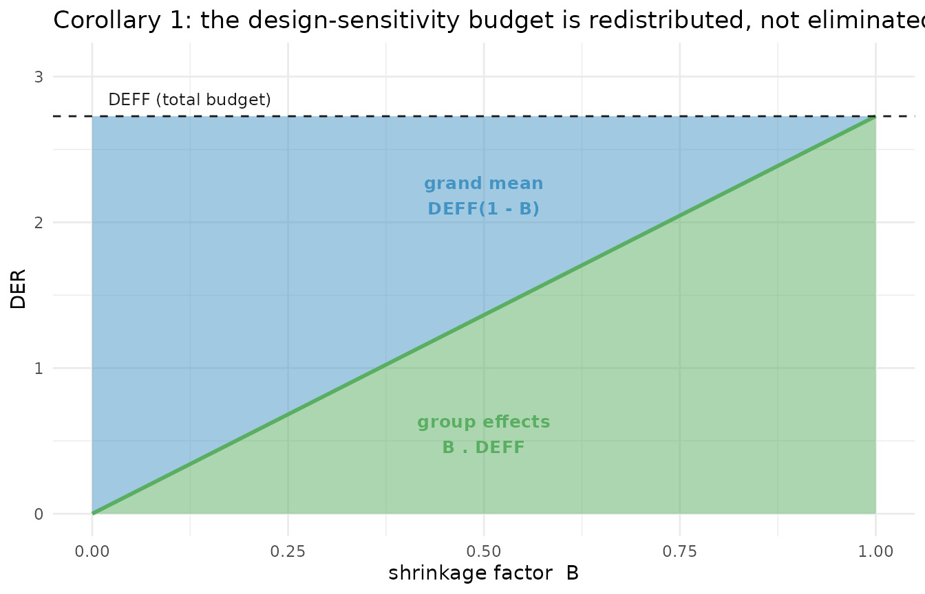
How the fixed design-sensitivity budget DEFF splits between the grand mean (blue) and the group effects (green) as the shrinkage factor B varies. The two shares always sum to DEFF (dashed line); shrinkage redistributes design sensitivity across the hierarchy rather than removing it.

At B = 0 the whole budget sits on the grand mean; at B = 1 it has all moved to the group effects; everywhere in between the split is exactly \mathrm{DEFF}(1-B) : B\,\mathrm{DEFF}.

Note. The conservation law is proven for the balanced conjugate Gaussian class under common \mathrm{DEFF}. Whether an analogous identity survives to unbalanced, non-Gaussian, or deeper hierarchies is open (paper, Discussion).

Empirical verification

We now check the closed forms against the software’s exact sandwich computation on nsece_demo — binomial, N = 6785, J = 51 states, \mathrm{DEFF} = 2.728 — with the design-PSU target (cluster = nsece_demo$psu). The demo is binomial rather than Gaussian, so the theorems apply only as a linearized approximation; the point is to see the mechanism reproduce, not to claim machine-precision equality.

result <- der_compute(
  nsece_demo$draws,
  y           = nsece_demo$y,
  X           = nsece_demo$X,
  group       = nsece_demo$group,
  weights     = nsece_demo$weights,
  cluster     = nsece_demo$psu,          # design-based target; NEVER psu =
  family      = "binomial",
  sigma_theta = nsece_demo$sigma_theta,
  param_types = nsece_demo$param_types
)

der_decompose(): the closed-form ingredients

der_decompose() returns, for every parameter, the design effect used, the shrinkage B, the between-group share R_k, the finite-group factor \kappa, and the resulting predicted DER — alongside the empirically computed der.

dc <- der_decompose(result)
head(dc, 6)
#>      param param_type       der deff_used    B_used        R_k     kappa
#> 1  beta[1] fe_between 0.2626885  2.727828        NA 0.93273657        NA
#> 2  beta[2]  fe_within 2.6894416  2.727828        NA 0.01430246        NA
#> 3  beta[3] fe_between 0.3430527  2.727828        NA 0.92282567        NA
#> 4 theta[1]         re 3.3858856  3.479991 0.6441524         NA 0.9467869
#> 5 theta[2]         re 0.6759045  2.417686 0.6072076         NA 0.9515495
#> 6 theta[3]         re 1.1182861  1.878577 0.5847477         NA 0.9540496
#>   der_predicted
#> 1     0.1834831
#> 2     2.6888138
#> 3     0.2105183
#> 4     2.1223599
#> 5     1.3969105
#> 6     1.0480173

Look first at the three fixed effects. The within-group covariate is beta[2] (poverty_cwc; in package output the poverty covariate is column 2, not column 1):

dc[dc$param_type != "re",
   c("param", "param_type", "der", "deff_used", "R_k", "der_predicted")]
#>     param param_type       der deff_used        R_k der_predicted
#> 1 beta[1] fe_between 0.2626885  2.727828 0.93273657     0.1834831
#> 2 beta[2]  fe_within 2.6894416  2.727828 0.01430246     2.6888138
#> 3 beta[3] fe_between 0.3430527  2.727828 0.92282567     0.2105183

This is Theorem 1 working exactly as advertised:

• beta[2] (within, Tier I-a): R_k \approx 0.014 — almost no between-group content, so \mathrm{DER}_{\beta_k} \approx \mathrm{DEFF}. The empirical der is 2.689 and the predicted value is 2.689: a within-group coefficient inherits essentially the whole design effect.
• beta[1] and beta[3] (between, Tier I-b): R_k \approx 0.93 — almost all between-group content, so both are pulled down into the shielded end of the band, with der 0.263 and 0.343 respectively. These are below 1: correcting them would wrongly narrow already-calibrated intervals.

The beta[2] agreement is the cleanest demonstration in the package that a pure within-group coefficient sits at R_k \approx 0 and inherits the full \mathrm{DEFF}.

Note. der_decompose() reports der_predicted using each parameter’s own Kish deff_used (here 2.728). The companion der_theorem_check() below scores Theorem 1 against the mean design effect (2.595, the fitted mean_deff), so its der_theorem1 for beta[2] reads about 2.595 rather than 2.689. Both are legitimate; they differ only in which \mathrm{DEFF} estimate stands in for the common value the theorem assumes.

For the random effects, der_decompose() populates B and \kappa (and leaves R_k as NA, since R_k is a fixed-effect concept):

re <- dc[dc$param_type == "re", ]
head(re[, c("param", "der", "deff_used", "B_used", "kappa", "der_predicted")], 4)
#>      param       der deff_used    B_used     kappa der_predicted
#> 4 theta[1] 3.3858856  3.479991 0.6441524 0.9467869      2.122360
#> 5 theta[2] 0.6759045  2.417686 0.6072076 0.9515495      1.396910
#> 6 theta[3] 1.1182861  1.878577 0.5847477 0.9540496      1.048017
#> 7 theta[4] 2.2098098  2.745753 0.7195228 0.9334392      1.844132

Here B \approx 0.58-0.64 and \kappa \approx 0.95, matching Theorem 2: theta[1], for instance, predicts B \cdot \mathrm{DEFF} \cdot \kappa \approx 2.12. But note the empirical der for theta[1] is 3.386 against a predicted 2.122 — a large gap. That is expected, and it is a data limitation, not a theory failure.

Key insight. This example is using the design-PSU target, so the random-effect gaps are best read as linearized-theory approximation error: the demo is binomial, groups are unbalanced, and the design effects are heterogeneous across states. Read the random-effect results tier-wise — the median RE DER is 1.311, comfortably in the Tier II range — not state-by-state.

Under a model-group target there is an additional estimator limitation: each state contributes only one centered score-total contrast to its own meat entry. That one-contrast issue belongs to the model-group target, not to the design-PSU computation shown here.

der_theorem_check(): scoring the closed forms

der_theorem_check() puts the empirical DER next to the theorem-predicted value and reports which theorem was used and the relative error.

tc <- der_theorem_check(result)
head(tc, 6)
#>      param param_type der_empirical der_theorem1 der_theorem2 relative_error
#> 1  beta[1] fe_between     0.2626885    0.3781171           NA     0.43941210
#> 2  beta[2]  fe_within     2.6894416    2.5952698           NA     0.03501540
#> 3  beta[3] fe_between     0.3430527    0.3781171           NA     0.10221260
#> 4 theta[1]         re     3.3858856           NA     2.122360     0.37317436
#> 5 theta[2]         re     0.6759045           NA     1.396910     1.06672753
#> 6 theta[3]         re     1.1182861           NA     1.048017     0.06283619
#>          theorem_used
#> 1 Theorem 1 (between)
#> 2  Theorem 1 (within)
#> 3 Theorem 1 (between)
#> 4      Theorem 2 (RE)
#> 5      Theorem 2 (RE)
#> 6      Theorem 2 (RE)

The fixed-effect rows confirm the pattern: beta[2] (within) is scored against Theorem 1’s within branch with small relative error, while the between effects beta[1]/beta[3] are scored against the between branch. The random-effect rows use Theorem 2 and, per the caveat above, show larger per-state relative errors because the design-PSU demo is a finite, unbalanced, binomial approximation to the balanced Gaussian theorem — theta[2] is the worst offender in the first few rows.

The conservation law is attached as an attribute, evaluated on the fitted quantities:

cl <- attr(tc, "conservation_law")
cl
#> $der_mu
#>   beta[1] 
#> 0.2626885 
#> 
#> $der_theta_cond
#> [1] 2.227894
#> 
#> $der_theta_marginal_mean
#> [1] 1.610739
#> 
#> $der_theta_mean
#> [1] 1.610739
#> 
#> $conservation_sum
#>  beta[1] 
#> 2.490582 
#> 
#> $deff_mean
#> [1] 2.59527
#> 
#> $relative_error
#>    beta[1] 
#> 0.04033774

The identity to check is \mathrm{DER}_\mu + \mathrm{DER}_\theta^{\mathrm{cond}} = \mathrm{DEFF}. The attribute reports der_mu (the grand-mean DER, here the beta[1] intercept), der_theta_cond (the conditional theorem term, computed from B_j \mathrm{DEFF}_j), their conservation_sum, and deff_mean for comparison. It also reports der_theta_marginal_mean, the empirical mean of the fitted random-effect DERs. The marginal mean is useful as an empirical diagnostic, but it is not the conditional term in the conservation identity.

On this binomial demo the conditional sum and \mathrm{DEFF} agree only approximately — the relative_error field quantifies the gap — because the model is not Gaussian, the groups are unbalanced, and the design effects are heterogeneous. The identity is exact only in the balanced Gaussian world the theorem inhabits; the demo shows the mechanism, not machine-precision equality.

When the formulas diverge

The closed forms are exact under (C1)-(C3) and the common-\mathrm{DEFF} clause. Two departures, both present in real applications and partly in the demo, move the software’s exact sandwich away from the simple predictions:

• Heterogeneous design effects (\mathrm{DEFF}_j not common). Balance forces a common B but never a common \mathrm{DEFF}. When the within-group design effects differ, Theorem 1’s \mathrm{DEFF} is replaced by \mathbf{M} = \sum_j \mathrm{DEFF}_j\, \mathbf{C}_j^{(d)} with \mathbf{C}_j^{(d)} = \mathbf{W}_j + \tfrac{(1 - B_j)^2}{a_j}\mathbf{b}_j\mathbf{b}_j^{\mathsf{T}} (distillation S-B.1), and the random-effect DER depends on the whole ensemble \{(B_j, \mathrm{DEFF}_j)\} rather than a naive per-group product (distillation S-B.3).
• Unbalanced groups (n_j not common). Then B_j varies too, and the single band [\mathrm{DEFF}(1-B),\ \mathrm{DEFF}] becomes a family of bands. The ensemble-exact expressions still hold; the two-number summary does not.

The software always computes the exact sandwich, so der_decompose() and der_theorem_check() remain correct diagnostics regardless. The closed forms are best read as the interpretive skeleton — they tell you which direction each tier moves and why — with the ensemble forms of distillation S-B.1-S-B.3 as the exact statement when balance or common \mathrm{DEFF} fails.

What’s next?

• To see how these tiers turn into a classification and a selective correction — the four-tier table, the threshold c_0, and block-Cholesky CCC — read vignette("theory-classification-correction").
• For the bread and meat behind the sandwich the theorems decompose — penalized Hessian, cluster-aggregated meat, weight conventions — see vignette("theory-sandwich").
• For the DER definition and the three regimes that motivate all of this, see vignette("theory-der").
• To watch the decomposition play out on a full worked example, see the applied Case Study.

References

• Lee, J., Williams, M. R., & Savitsky, T. D. (2026). Design Effect Ratios for Bayesian Survey Models: A Diagnostic Framework for Identifying Survey-Sensitive Parameters. Journal of Survey Statistics and Methodology (submitted).
• Fay, R. E., & Herriot, R. A. (1979). Estimates of income for small places: An application of James-Stein procedures to census data. Journal of the American Statistical Association, 74(366), 269-277.
• Kish, L. (1965). Survey Sampling. Wiley.