
Comparing the three fitting methods
JoonHo Lee
2026-09-11
Source:vignettes/a4-comparing-methods.Rmd
a4-comparing-methods.RmdAbstract
pvstackr has three fitting methods, stack_direct,
per_pv and stack_psis. This article
describes how they differ, lines up three example fits with
pv_compare_methods(), and reads the estimates and the
agreement diagnostics of the comparison. It ends with two
cautions, on the standard errors and on the Pareto k-hat values of
stack_psis, and with pvstackr’s recommendation for
choosing a method.
pvstackr fits a model to plausible-value data with one of three
methods: stack_direct (the default), per_pv
and stack_psis.
The example compares three fits of the small synthetic data set
bundled with pvstackr. The stack_direct fit is the example
fit that ships with the package; Getting started with
pvstackr describes how it was made. The per_pv fit is
made from random numbers near the example estimates instead of posterior
draws, because a real per_pv fit needs one Bayesian fit per
plausible value. The stack_psis fit gets placeholder
importance weights and Pareto \(\hat
k\) values, both explained in the three
methods, that no program computed; since no program is named,
pvstackr blocks the fit (PSIS status
provenance_incomplete). The numbers therefore show the
layout of the output and say nothing about how the methods compare on
real data.
The three methods
All three methods report only the fixed effects, and all three combine the results for the \(M\) plausible values with Rubin’s rules (Rubin 1987), so their standard errors include the variation between plausible values. They differ in the number of Bayesian fits they need and in where the variance within a plausible value comes from:
| Method | Bayesian fits | Variance within a plausible value | Intervals | Bundled engine |
|---|---|---|---|---|
stack_direct (default) |
1 | BRR–Fay replicate weights, through the target | coverage-claimable only with an external Barnard–Rubin target, otherwise descriptive | brms, with
pv_control(backend = "brms")
|
per_pv |
\(M\) | posterior draws of each fit | always descriptive | none |
stack_psis |
1 | posterior draws of the stacked fit, reweighted | always descriptive | none |
A coverage-claimable interval is one that pvstackr’s reporting rule
lets you read as a confidence interval with nominal coverage
(coverage_claim_allowed = TRUE); Reading and reporting
the results gives the rule and the interval_role label
of each case.
stack_direct fits one model to the stacked data (\(M\) copies of the data, one per plausible
value) and calibrates its fixed-effect draws to the target from
pv_brr_target(); its estimate table reports the target’s
estimates, standard errors and degrees of freedom. The target itself
takes \(M(R + 1)\) weighted
least-squares fits, which need no sampler. The full analysis workflow
describes both steps.
per_pv combines one Bayesian fit per plausible value.
You supply the fits, either as their posterior draws
(per_pv_draws) or as your own fitting functions, which
pvstackr calls once per plausible value. pvstackr does not pass the
survey weights to these functions, so a weighted fit has to take them
from the data. Scale them as pvstackr scales the weights of the stacked
fit, by dividing the final weight by its mean: with flat priors on the
coefficients, the posterior means do not depend on the scale of the
weights, but the posterior standard deviations do. PISA final weights
count the students that each sampled student represents (OECD 2024), so fits that use them unscaled give
posterior standard deviations that are far too small, and
per_pv standard errors that are too small.
?pv_fit_reference lists what these functions receive and
return. pvstackr also collects no sampler diagnostics from them: a
per_pv fit always has status "ok", so check
the convergence of each fit yourself.
stack_psis reweights the draws of one fit to the stacked
data toward each plausible value. For each plausible value you supply
importance weights and a Pareto \(\hat
k\) value, computed outside pvstackr, for example by Pareto
smoothed importance sampling (PSIS) with the loo package (Vehtari et al. 2017, 2024); \(\hat k\) shows how reliable the reweighted
estimates are. pvstackr computes no part of PSIS: it divides each column
of weights by its sum, reweights the draws and combines the results with
Rubin’s rules. It blocks the fit unless every \(\hat k\) is below
psis_k_threshold in pv_control() (0.7 by
default) and the program that made the weights is named with
psis_producer and psis_producer_version.
?pv_fit_stack_psis lists the inputs.
The number of Bayesian fits says how many samplers run, not how long the analysis takes.
Running a comparison
pv_compare_methods() takes two or more finished fits and
lines up their estimate tables by fixed-effect name; it fits no model
itself. The three fits below have the same fixed effects,
b_Intercept, b_x and b_female.
The stack_direct fit is read from the package. The other
two are made from draws passed in directly:
pv_fit_reference(), which runs the per_pv
method, takes a list of draw matrices, one per plausible value, and
pv_fit_stack_psis(), which runs stack_psis,
takes a matrix of stacked draws with the weights and the \(\hat k\) values. No sampler runs and no
PSIS is computed. The stack_psis call names no program,
because no program made its weights.
fe <- c("b_Intercept", "b_x", "b_female")

fit_direct <- readRDS(
  system.file("extdata", "examples", "pisa_tiny_stack_direct.rds",
              package = "pvstackr")
)$fit

# Made-up draws for the per_pv fit: for each plausible value, 300 random values
# per fixed effect, with standard deviation 2, around 458, 47 and 2, near the
# example estimates. They stand in for posterior draws; no model was fitted.
set.seed(1)
mk <- function(mu) {
  d <- matrix(rnorm(300 * 3, sd = 2), ncol = 3, dimnames = list(NULL, fe))
  sweep(d, 2L, mu, "+")
}

fit_per_pv <- pv_fit_reference(
  per_pv_draws = list(PV1READ = mk(c(458, 47, 2)),
                      PV2READ = mk(c(458, 47, 2))),
  control      = pv_control(method = "per_pv")
)

# Made-up stacked draws with equal placeholder weights and Pareto k-hat values
# of 0.2. No PSIS was run, so no program is named, and pvstackr blocks the fit
# (its PSIS status is provenance_incomplete).
sd_mat <- mk(c(458, 47, 2))
fit_psis <- pv_fit_stack_psis(
  stacked_draws = sd_mat,
  pv_cols       = c("PV1READ", "PV2READ"),
  psis_weights  = matrix(1 / nrow(sd_mat), nrow = nrow(sd_mat), ncol = 2),
  pareto_k      = c(0.2, 0.2),
  control       = pv_control(method = "stack_psis")
)
The comparison is one call:
cmp <- pv_compare_methods(
  stack_direct = fit_direct,
  per_pv       = fit_per_pv,
  stack_psis   = fit_psis
)

cmp
#> pvstackr method comparison
#>   reference: per_pv
#>   methods: stack_direct=stack_direct, per_pv=per_pv, stack_psis=stack_psis
#>   fixed effects: 3
#>   blocked: stack_psis
#>   provenance note: Agreement bands are descriptive; shared target, pooling, or source metadata should not be read as independent corroboration.
#>   interval note: intervals are descriptive rather than coverage-claimable.
The print first names the reference fit, per_pv, from
which the differences in the comparison are taken. By default it is the
first per_pv fit that is not blocked, or, without one, the
first fit that is not blocked; choose another with the argument
reference_method. It then lists the label and the method of
each fit, the number of fixed effects (3) and the blocked fit,
stack_psis. The line provenance note: appears
in every comparison; the agreement diagnostics
explain it. The line interval note: says that the compared
intervals are descriptive.
The comparison has a row for each fit and each fixed effect that
appears in any of the fits. A blocked fit keeps its rows, with
NA values and its reason code, so that it stays visible in
the comparison.
The estimates side by side
get_estimates() on a comparison returns one row per fit
and fixed effect, here \(3 \times 3 =
9\) rows. For each row it gives the fit’s estimate, standard
error, degrees of freedom, interval and interval labels, the method,
status and reason codes of the fit, and the estimate and standard error
of the reference fit with the differences from them (see the agreement diagnostics); the source labels and
checksums of the fits are in get_diagnostics(). The columns
below put each estimate next to its interval and the two columns that
say how the interval can be read:
est <- get_estimates(cmp)

est[, c("method_label", "term", "estimate", "se",
        "conf_low", "conf_high",
        "interval_role", "coverage_claim_allowed")]
#>   method_label        term   estimate        se   conf_low  conf_high
#> 1 stack_direct b_Intercept 457.894088 1.2873118 442.318045 473.470132
#> 2 stack_direct         b_x  46.883361 0.3717929  44.414570  49.352151
#> 3 stack_direct    b_female   2.143702 3.5550309 -41.606872  45.894276
#> 4       per_pv b_Intercept 457.980857 1.9931772 454.074152 461.887563
#> 5       per_pv         b_x  47.038417 2.0556785  43.009330  51.067504
#> 6       per_pv    b_female   1.869331 2.1659676  -2.375888   6.114549
#> 7   stack_psis b_Intercept         NA        NA         NA         NA
#> 8   stack_psis         b_x         NA        NA         NA         NA
#> 9   stack_psis    b_female         NA        NA         NA         NA
#>               interval_role coverage_claim_allowed
#> 1 descriptive_classic_rubin                  FALSE
#> 2 descriptive_classic_rubin                  FALSE
#> 3 descriptive_classic_rubin                  FALSE
#> 4   reference_classic_rubin                  FALSE
#> 5   reference_classic_rubin                  FALSE
#> 6   reference_classic_rubin                  FALSE
#> 7                      <NA>                     NA
#> 8                      <NA>                     NA
#> 9                      <NA>                     NA
The stack_direct rows hold the numbers of the example
fit, which are those of its target. The per_pv estimates
are close to them only because the made-up draws were placed around 458,
47 and 2, and their standard errors, about 2, come from the standard
deviation of those draws. The stack_psis rows are
NA because that fit is blocked.
Two columns say how each interval can be read:
-
interval_roleisdescriptive_classic_rubinforstack_direct, because the example target uses the classic Rubin degrees of freedom, andreference_classic_rubinforper_pv. It isNAfor the blockedstack_psisrows; astack_psisfit with estimates haspsis_classic_rubinorpsis_barnard_rubin. -
coverage_claim_allowedisFALSEfor the two fits with estimates andNAfor the blocked one. With a target made with Barnard–Rubin degrees of freedom, thestack_directrows would haveTRUE; theper_pvandstack_psisrows haveFALSEwhatever their degrees of freedom.
The intervals also differ in width. For the slope of
x:
bx <- est[est$term == "b_x",
          c("method_label", "se", "conf_low", "conf_high")]
bx$width <- bx$conf_high - bx$conf_low
bx
#>   method_label        se conf_low conf_high    width
#> 2 stack_direct 0.3717929 44.41457  49.35215 4.937582
#> 5       per_pv 2.0556785 43.00933  51.06750 8.058174
#> 8   stack_psis        NA       NA        NA       NA
The width of an interval depends on the standard error and on the
degrees of freedom. The stack_direct interval is 4.9 points
wide although its standard error is 0.37, because the example target has
only 1.40 classic degrees of freedom for b_x. The
per_pv interval is 8.1 points wide, about four times its
standard error of 2.06, which comes from the made-up draws. Neither
width says anything about real data. The blocked stack_psis
row has no interval.
The figure shows the estimates and intervals of the two slopes; the
intercept, about 458, is left out because its scale would compress the
axis. The blocked stack_psis fit has nothing to draw.
slopes  <- est[est$term != "b_Intercept",
               c("method_label", "term", "estimate", "conf_low", "conf_high")]
slopes  <- slopes[is.finite(slopes$estimate), , drop = FALSE]
methods <- unique(slopes$method_label)
terms   <- sort(unique(slopes$term))

offsets <- setNames(seq(-0.18, 0.18, length.out = length(methods)), methods)
cols    <- setNames(c("#1f6f9c", "#f2c14e", "grey45")[seq_along(methods)], methods)

xlim <- range(c(slopes$conf_low, slopes$conf_high, 0), na.rm = TRUE)

op <- par(mar = c(4.5, 7, 1, 1))
plot(
  NA, xlim = xlim, ylim = c(0.5, length(terms) + 0.5),
  yaxt = "n", ylab = "",
  xlab = "Coefficient (synthetic reading-score points)"
)
abline(v = 0, lty = 2, col = "grey50")
for (mlab in methods) {
  sub <- slopes[slopes$method_label == mlab, ]
  yy  <- match(sub$term, terms) + offsets[[mlab]]
  segments(sub$conf_low, yy, sub$conf_high, yy, lwd = 2, col = cols[[mlab]])
  points(sub$estimate, yy, pch = 19, cex = 1.3, col = cols[[mlab]])
}
axis(2, at = seq_along(terms), labels = terms, las = 1)
legend("topleft", legend = methods, col = cols, pch = 19, lwd = 2,
       bty = "n", cex = 0.9)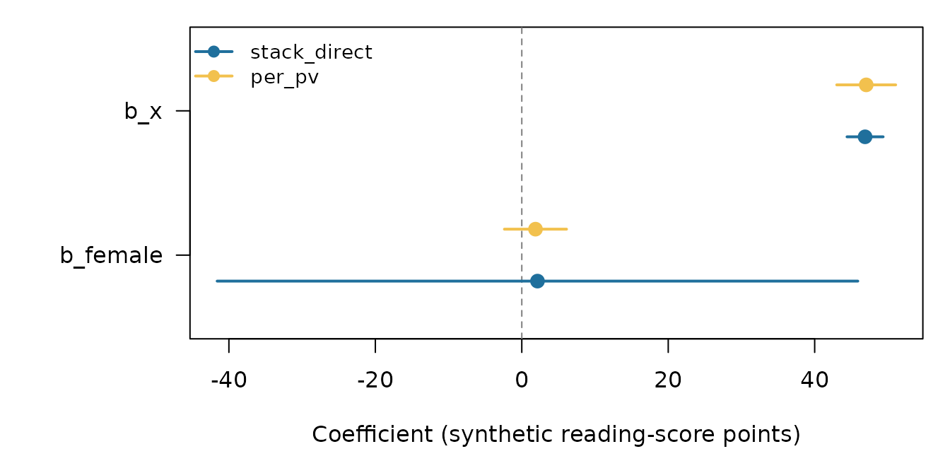
Estimates and 95% intervals of the two slopes, b_x and b_female, from the stack_direct and per_pv fits. The blocked stack_psis fit has no estimates to draw. The dashed line marks zero. The per_pv values come from made-up draws.
par(op)Both intervals for b_x lie well above zero, and both
intervals for b_female include it. The
stack_direct interval for b_female, from about
−42 to 46, is much wider than the per_pv one, from about −2
to 6, for the reasons given above.
On real data, the estimates of the three methods are close when they
all fit the same survey-weighted model. A stack_direct fit
reports the target’s \(\bar\beta\), the
average over the plausible values of the survey-weighted least-squares
estimates. A per_pv fit reports the average of the
posterior means of your fits. If each of these fits is the same
survey-weighted regression, with the weights taken from the data and
flat priors on the fixed effects (in brms, write the intercept as
0 + Intercept, because its default prior on the intercept
is not flat), its posterior mean is the weighted least-squares estimate
for its plausible value, apart from Monte Carlo error; the
per_pv estimates then differ from \(\bar\beta\) only by that error.
The same holds for a stacked fit, which stack_direct
calibrates and stack_psis reweights. When its rows are
weighted by \(\tilde w_i/M\), where
\(\tilde w_i\) is the final survey
weight divided by its mean, the weighted least-squares estimate from the
stacked data equals \(\bar\beta\)
exactly in pvstackr’s model, a weighted linear regression without random
effects. The stacked fixed-effect point identity, Theorem 4.1 of the
companion preprint (Lee et al. 2026),
states the conditions for this equality, and One stacked fit and the Rubin point
estimate explains it. The reweighted means of
stack_psis approximate the posterior means for the separate
plausible values, and the Pareto \(\hat
k\) values show how reliable these approximations are (Vehtari et al. 2024). The standard errors are
another matter, which the first of the cautions
explains.
Agreement diagnostics
get_diagnostics() on a comparison returns a list:
dg <- get_diagnostics(cmp)
names(dg)
#> [1] "reference_method"   "methods"            "statuses"
#> [4] "blocked_methods"    "warning_methods"    "agreement"
#> [7] "method_diagnostics" "timing"             "target_overlap"
reference_method and methods repeat what
print() shows, statuses gives the status of
each fit, and blocked_methods and
warning_methods list the fits with status
"blocked" or "warning". timing
gives the number of model fits of each method and, when you pass times
that you measured with the argument timings, the elapsed
seconds; pvstackr does not time the fits itself. The other three
elements describe how the fits agree.
agreement has one row per fit.
max_abs_z_diff is the largest, over the fixed effects, of
the absolute difference between the fit’s estimate and the reference
estimate, divided by \(\sqrt{\mathrm{se}^2 +
\mathrm{se}_{\text{ref}}^2}\). max_abs_log_se_ratio
is the largest absolute log of the ratio of the fit’s standard error to
the reference standard error:
dg$agreement
#>         method method_label  status max_abs_z_diff max_abs_log_se_ratio n_terms
#> 1 stack_direct stack_direct      ok     0.07422425             1.710024       3
#> 2       per_pv       per_pv      ok     0.00000000             0.000000       3
#> 3   stack_psis   stack_psis blocked             NA                   NA       3
#>   n_available
#> 1           3
#> 2           3
#> 3           0
The reference fit, per_pv, has zeros. For
stack_direct, max_abs_z_diff is 0.07: the
estimates are close because the made-up per_pv draws were
placed near them. max_abs_log_se_ratio is 1.71 and comes
from b_x, whose stack_direct standard error,
0.37, is 0.18 times the per_pv one, 2.06. The blocked
stack_psis fit has no estimates (n_available
is 0) and therefore no values.
The estimate table of the comparison gives the same measures for each
row (estimate_diff, se_ratio and
abs_z_diff), and agreement_band groups
abs_z_diff by pvstackr’s cut-offs: "close"
below 0.1, "moderate" from 0.1, "different"
from 0.5, and "not_available" for a blocked fit. These
values describe how far apart the fits are; they are not a statistical
test. In a real comparison, max_abs_z_diff shows whether
the fits agree on the estimates and max_abs_log_se_ratio
how far their standard errors differ; the
cautions explain why the two need not go together.
target_overlap records whether fits share their
numbers:
str(dg$target_overlap)
#> List of 8
#>  $ shared_external_target      : logi FALSE
#>  $ shared_target_hash          : logi FALSE
#>  $ shared_pooling_hash         : logi FALSE
#>  $ shares_reference_target     : logi FALSE
#>  $ shares_reference_pooling    : logi FALSE
#>  $ shared_target_sources       : chr(0)
#>  $ independence_caveat_required: logi FALSE
#>  $ independence_caveat         : chr "Agreement bands are descriptive; shared target, pooling, or source metadata should not be read as independent corroboration."
Every flag is FALSE here: the stack_direct
fit has the target made by pv_brr_target(), the
per_pv fit has its own combination of its draws, and the
blocked fit has neither. The flags become TRUE when two or
more fits have the same target (shared_target_hash, and
shared_external_target when they are
stack_direct fits calibrated to the same target) or the
same combined result (shared_pooling_hash), or when a fit
has the target or the combined result of the reference fit
(shares_reference_target,
shares_reference_pooling).
shared_target_sources lists the source labels that two or
more fits have, and independence_caveat_required is
TRUE when any flag is TRUE or that list is not
empty. independence_caveat holds the text of the
provenance note: line.
Agreement between fits that share their numbers follows by
construction: two stack_direct fits calibrated to the same
target report the same estimates and standard errors, whatever their
draws. Even without shared numbers, fits of the same data and plausible
values are not independent, so their agreement does not confirm a
result.
method_diagnostics has one row per fit and many columns,
which ?pv_compare_methods lists; the chunk shows some of
them:
dg$method_diagnostics[, c("method_label", "interval_role",
                          "coverage_claim_allowed", "target_source",
                          "psis_status", "pareto_k_max", "n_fits")]
#>              method_label             interval_role coverage_claim_allowed
#> stack_direct stack_direct descriptive_classic_rubin                  FALSE
#> per_pv             per_pv   reference_classic_rubin                  FALSE
#> stack_psis     stack_psis                      <NA>                     NA
#>                       target_source           psis_status pareto_k_max n_fits
#> stack_direct external_brr_fay_rubin                  <NA>           NA      1
#> per_pv           per_pv_rubin_draws                  <NA>           NA      2
#> stack_psis                     <NA> provenance_incomplete          0.2      1
target_source labels where the numbers of a fit come
from: external_brr_fay_rubin for the target from
pv_brr_target() and per_pv_rubin_draws for
Rubin’s rules applied to the per_pv draws. It is
NA for the blocked fit. A stack_psis fit with
estimates has the label stack_psis_rubin_pooling but no
target object: get_target() returns NULL for
it. n_fits is the number of model fits: 1 for
stack_direct, \(M = 2\)
for per_pv and 1 for stack_psis. For the
blocked fit, psis_status is
"provenance_incomplete" because no program was named, and
pareto_k_max, the largest of the \(\hat k\) values supplied, is the 0.2 typed
into the example; pvstackr records it but cannot tell how it was
obtained.
pvstackr checks the \(\hat k\)
values against one cut-off, psis_k_threshold in
pv_control(): 0.7 by default, which is also the largest
value allowed. A stack_psis fit is blocked unless the \(\hat k\) of every plausible value is below
it. Choosing a method and
reading its intervals gives the cut-offs of the literature and how
to set psis_k_threshold to one of them.
Cautions in reading a comparison
Standard errors from the model and from the replicate weights
Fits that agree on the estimates can still differ in their standard
errors, because the methods take the variance within a plausible value
from different sources. The target of stack_direct takes it
from the BRR–Fay replicate weights, which PISA provides for estimating
the sampling variance under its design. In such a design, clustering
(students sampled within schools) and unequal weights usually increase
the sampling variance, while stratification reduces it (OECD 2024). per_pv and
stack_psis take the variance from the posterior draws of a
model. The draws reflect the clustering only as far as the model
includes it (a single-level regression treats the students as
independent), and weighting the likelihood by the survey weights does
not by itself make their variance design-based (Williams and Savitsky 2021). The two variances
can therefore differ even when the estimates agree. The example cannot
show this, because its per_pv standard errors come from the
made-up draws.
This difference is the reason for pvstackr’s reporting rule in the three methods. Close agreement between the estimates of two methods does not tell you which standard errors to report.
Pareto \(\hat k\) values check only the importance weights
For a stack_psis fit, a \(\hat
k\) below the cut-off of Vehtari et al.
(2024), \(\min(1 - 1/\log_{10} S,
0.7)\) for \(S\) draws,
indicates that the importance ratios for that plausible value pass this
diagnostic; the reliability of a weighted mean or covariance depends on
the Pareto \(\hat k\) of that quantity,
which can be larger (Vehtari et al. 2024, 7,
14). With fewer than about 2,000 draws this cut-off is below
pvstackr’s default of 0.7. It does not change where the variance comes
from: the standard errors of a stack_psis fit still come
from the posterior draws of the stacked model, as in the previous
caution.
pvstackr cannot check the \(\hat k\)
values either. It computes neither them nor the weights, so it asks you
to name the program that produced them, with psis_producer
and psis_producer_version, and records the name without
checking it: a producer name alone is not evidence that PSIS was run. In
the example the value 0.2 was typed in and no program is named, so the
fit stays blocked.
\(\hat k\) also depends on the data,
the model and the posteriors that the weights aim at, so check it in
every analysis. In the application of the companion preprint to PISA
2022, one stacked fit per country was reweighted, in the same way in
both countries, toward the posteriors of a model with a school random
intercept, with the survey weights placed in two stages; every \(\hat k\) was below 0.7 in the United States
and above it in Korea (Lee et al. 2026, sec. 6.4
and app. D.1). pvstackr 0.2.x does not fit that model, so these
values are not direct evidence about stack_psis fits of the
single-level model that pvstackr fits (Choosing a method and reading its
intervals gives the details).
Choosing a method
pvstackr recommends the following (a package rule, not a result of the companion preprint):
- Report a
stack_directfit. Its estimate table holds the numbers of the design-based target, its intervals are the only ones that can be coverage-claimable (with a Barnard–Rubin target), and it needs one Bayesian fit. - Use
per_pvto compare thestack_directestimates with one Bayesian fit per plausible value. Its intervals are descriptive, and pvstackr does not check the convergence of its fits. - Use
stack_psisonly as a check on a stacked fit, with importance weights and \(\hat k\) values from a PSIS program. Its intervals are descriptive as well.
The companion preprint notes that for a single, final, high-stakes model one fit per plausible value remains a sound default (Lee et al. 2026, sec. 7).
Reading and reporting the results explains the interval labels of every method and what to report for a fit. Among the Method articles, Choosing a method and reading its intervals compares the methods and their intervals in more detail, and One stacked fit and the Rubin point estimate explains the stacked fixed-effect point identity, whose proof is in the preprint.