Getting started with pvstackr

Abstract

pvstackr fits regression models to assessment data with plausible values, such as PISA, and reports the fixed-effect coefficients. This article shows how to install the package and write the pv_fit() call for the default method, stack_direct. It then reads a precomputed fit of the bundled synthetic data with print(), get_estimates() and a coefficient plot, and shows the columns of the estimate table that say whether pvstackr’s reporting rule lets you read an interval as a confidence interval with nominal coverage.

library(pvstackr)

Plausible values

Large-scale assessments such as PISA do not publish a single test score for each student. Because proficiency is not observed directly, each student receives a set of plausible values: $M$ draws from that student’s posterior distribution of proficiency (Mislevy 1991; von Davier et al. 2009). The standard analysis fits the model once for each plausible value, with the survey weights and a replicate-weight estimate of each fit’s sampling variance, and combines the $M$ results with Rubin’s rules for multiple imputation (Rubin 1987). An analysis that uses only PV1 omits the between-imputation variance (the variation of the estimates across plausible values), so its standard errors are too small.

What pvstackr computes

The default method, stack_direct, fits one model to the stacked data ($M$ copies of the data, one per plausible value) and then calibrates the fixed-effect draws of that fit to the target: the estimates, covariance matrix and degrees of freedom that pv_brr_target() computes with the standard analysis described above (a survey-weighted regression for each plausible value, the BRR–Fay replicate weights for the sampling variance of the coefficients, and Rubin’s rules to combine the results). The calibration transforms the draws so that their mean and covariance equal those of the target. The setting center = "target" in pv_control(), the default and the only value stack_direct accepts, centers the calibrated draws on the target’s estimates, so the reported estimates, standard errors and degrees of freedom are those of the target: the Bayesian fit does not change them. It supplies the calibrated draws, which can be used for quantities derived from the coefficients, such as the difference between two of them, and diagnostics that show how closely the fit agrees with the target. stack_direct needs one Bayesian fit where a Bayesian analysis of each plausible value needs $M$, but that fit has $M$ times as many rows.

pv_fit() also offers per_pv, which fits one model per plausible value and combines the results with Rubin’s rules, and stack_psis, which reweights one stacked fit toward each plausible value with importance weights that you supply. Both take the variance within each plausible value from the model’s posterior draws rather than from the replicate weights, so their intervals are always descriptive. The stack_direct model is a linear regression weighted by the survey weights; stack_direct, stack_psis and pv_brr_target() stop with an error if the formula contains a random-effect term such as (1 | school). Only the fixed-effect coefficients (intercept and slopes) are reported; other parameters of the model, such as the residual standard deviation sigma, are neither calibrated nor reported.

By pvstackr’s reporting rule, only a stack_direct fit whose target uses Barnard–Rubin degrees of freedom has intervals that can be read as confidence intervals with nominal coverage; the example fit uses the classic Rubin degrees of freedom, so its intervals are descriptive (see the section on intervals).

The examples below read a fit of the small synthetic data set bundled with the package, computed in advance (the example data and fit); the article fits no model, so it runs in seconds.

Installing pvstackr

Install pvstackr from GitHub, for example with the pak package:

# install.packages("pak")
pak::pak("joonho112/pvstackr")

Then load it (the first chunk of this article did so):

library(pvstackr)

Reading the example fit needs no modeling engine. A fit on your own data needs one: either the engine bundled with pvstackr or fitting functions of your own. The bundled engine fits the model with the brms package, so it needs brms and posterior installed.

Calling `pv_fit()`

pv_fit() fits a model with any of the three methods. For stack_direct, the default, a call on your own data has this form. The chunk is not run, because this article computes no target and uses no engine:

fit <- pv_fit(
  data    = your_data,
  formula = OUTCOME ~ x + female,   # OUTCOME stands for each plausible value
  target  = your_target,            # made by pv_brr_target()
  method  = "stack_direct",
  control = pv_control(method = "stack_direct", backend = "brms")
)

data is a data frame with one row per student: the plausible-value columns, the final survey weight, the replicate weights and the covariates.
formula has the placeholder OUTCOME on the left-hand side. pvstackr replaces it by each plausible-value column in turn (PV1READ, PV2READ, …), so you write the model once instead of $M$ times.
target is the design-based target, made by pv_brr_target() from the same data and formula (The full analysis workflow shows the call); pv_fit() stops with an error when the data or the formula differ from those of the target.
control holds the settings of the fit, made by pv_control() with the same method; pv_fit() stops with an error when the two differ. backend = "brms" selects the engine bundled with pvstackr; with the default, backend = "none", a stack_direct fit stops with an error unless you pass fitting functions of your own.

Instead of the bundled engine you can pass three functions of your own to pv_fit(): fit_function, draws_function and diagnose_function. The full analysis workflow describes what each one receives and returns.

The example data and fit

pvstackr includes a small synthetic data set and a stack_direct fit made from it, so that the examples run without PISA files. Load both:

pisa_tiny <- read.csv(
  system.file("extdata", "pisa_tiny.csv", package = "pvstackr")
)

fit <- readRDS(
  system.file("extdata", "examples", "pisa_tiny_stack_direct.rds",
              package = "pvstackr")
)$fit

The data set, pisa_tiny, has 12 students in three schools of one made-up country (CNT is "SYN"). Besides the student and school identifiers CNTSTUID and CNTSCHID, it has a continuous covariate x, a 0/1 indicator female, two plausible values for reading, PV1READ and PV2READ ($M = 2$), the final survey weight W_FSTUWT and four replicate weights, W_FSTURWT1 to W_FSTURWT4 ($R = 4$):

str(pisa_tiny)
#> 'data.frame':    12 obs. of  12 variables:
#>  $ CNT       : chr  "SYN" "SYN" "SYN" "SYN" ...
#>  $ CNTSCHID  : chr  "sch01" "sch01" "sch01" "sch01" ...
#>  $ CNTSTUID  : chr  "stu01" "stu02" "stu03" "stu04" ...
#>  $ x         : num  -1.4 -1.1 -0.7 -0.4 -0.1 0.2 0.5 0.8 1 1.3 ...
#>  $ female    : int  1 0 1 0 1 0 0 1 1 0 ...
#>  $ PV1READ   : int  398 410 423 437 451 466 480 494 507 522 ...
#>  $ PV2READ   : int  402 408 427 435 454 463 483 492 511 519 ...
#>  $ W_FSTUWT  : num  1 1.08 0.94 1.12 1.03 1.19 0.91 1.25 1.1 0.98 ...
#>  $ W_FSTURWT1: num  0.82 1.28 1.01 1.09 0.96 1.35 0.84 1.42 1.21 0.89 ...
#>  $ W_FSTURWT2: num  1.18 0.91 0.85 1.31 1.12 1.02 0.76 1.5 0.99 1.08 ...
#>  $ W_FSTURWT3: num  1.05 1.02 1.12 0.98 1.25 1.14 0.87 1.3 1.34 1.03 ...
#>  $ W_FSTURWT4: num  0.95 1.17 0.93 1.24 1.01 1.31 1.07 1.08 0.88 1.19 ...

The values were made up for the examples and the package tests; the data contain no PISA records, so the numbers illustrate the output and support no substantive conclusion. PISA 2022 provides ten plausible values per domain and 80 replicate weights (OECD 2024); the example has two and four, which keeps the objects small. Real PISA data: access, memory and reproducibility describes how to work with real PISA files.

The example fit was not made by a sampler. Its target was computed from pisa_tiny by pv_brr_target() with the classic degrees of freedom, and the fit was made with fitting functions written for the example, which ignore the data and return draws built from the target’s estimates and standard errors together with a typed-in sampler record. The fit was saved without its calibrated draws (return_draws = FALSE in pv_control()).

Because its draws were built around the target, the stacked fit agrees with the target by construction. The diagnostics that compare the two show differences of about $10^{-14}$ target standard errors, where a fit made by a sampler would differ by its Monte Carlo error (Reading and reporting the results shows these values). The example therefore shows what the output of a fit looks like, not how well the method works.

Reading the fit

The overview from `print()`

print() shows an overview of the fit:

print(fit)
#> pvstackr fit
#>   method: stack_direct
#>   status: ok
#>   fixed effects: 3
#>   target: external_brr_fay_rubin
#>   draws: not retained
#>   diagnostics: preflight, sampler, sampler_gate, stack_fit, stack_fit_warnings, ccc
#>   interval note: intervals are descriptive rather than coverage-claimable.

The first lines give the method, the status and the number of fixed effects. The target line gives the source of the target: external_brr_fay_rubin marks a target made by pv_brr_target() from the BRR–Fay replicate weights and Rubin’s rules. The draws line says that the calibrated draws were not kept, and the diagnostics line names the parts that get_diagnostics(fit) returns. The last line notes that the intervals are descriptive, which Reading the intervals explains.

status: ok means that none of pvstackr’s checks raised a warning or blocked the fit. It is not a statement that a sampler converged. For a stack_direct fit the checks cover the sampler diagnostics (R-hat, effective sample sizes, divergent transitions), the difference between the stacked fit and the target before the calibration, the numerical stability of the calibration, and any prior that you set (an explicit prior always gives a warning). A fit with status "warning" still has estimates, and print() then lists the reason codes; a fit with status "blocked" has an empty estimate table. “Status and checks” in ?pvstackr_object_contracts gives the thresholds of the checks.

The estimate table

get_estimates() returns the estimate table, a data frame with one row per fixed effect. The chunk shows 8 of its 17 columns:

est <- get_estimates(fit)

est[, c("term", "estimate", "se", "df",
        "conf_low", "conf_high",
        "interval_role", "coverage_claim_allowed")]
#>          term   estimate        se       df  conf_low conf_high
#> 1 b_Intercept 457.894088 1.2873118 1.021194 442.31804 473.47013
#> 2         b_x  46.883361 0.3717929 1.402308  44.41457  49.35215
#> 3    b_female   2.143702 3.5550309 1.013730 -41.60687  45.89428
#>               interval_role coverage_claim_allowed
#> 1 descriptive_classic_rubin                  FALSE
#> 2 descriptive_classic_rubin                  FALSE
#> 3 descriptive_classic_rubin                  FALSE

The terms are the intercept b_Intercept and the slopes b_x and b_female: pvstackr names each coefficient after its column of the model matrix, with the prefix b_. In these synthetic data the intercept is about 458 points, the slope of x about 47 points per unit of x, and the coefficient of female about 2 points. se is the standard error, and df the degrees of freedom used for the interval from conf_low to conf_high. The last two columns say how each interval can be read. Reading and reporting the results describes all 17 columns.

A plot of the slopes

The plot shows the two slopes with their intervals. The intercept is left out, since at about 458 points it would stretch the axis, and a dashed line marks zero:

slopes <- est[est$term != "b_Intercept", ]
slopes <- slopes[order(slopes$term), ]

y    <- seq_len(nrow(slopes))
xlim <- range(c(slopes$conf_low, slopes$conf_high, 0))

op <- par(mar = c(4.5, 7, 1, 1))
plot(
  slopes$estimate, y,
  xlim = xlim, ylim = c(0.5, nrow(slopes) + 0.5),
  yaxt = "n", ylab = "",
  xlab = "Coefficient (synthetic reading-score points)",
  pch = 19, cex = 1.4, col = "#1f6f9c"
)
abline(v = 0, lty = 2, col = "grey50")
segments(slopes$conf_low, y, slopes$conf_high, y, lwd = 2, col = "#1f6f9c")
points(slopes$estimate, y, pch = 19, cex = 1.4, col = "#1f6f9c")
axis(2, at = y, labels = slopes$term, las = 1)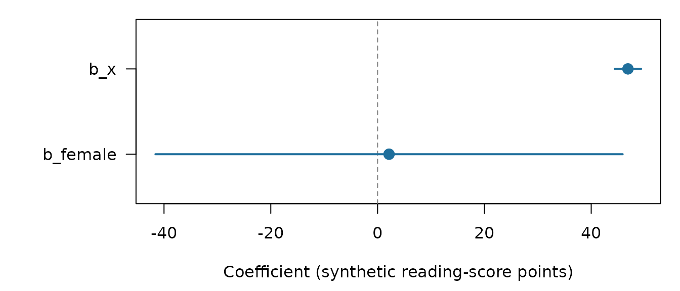

Dot-and-interval plot of the two slopes of the example fit, on a horizontal axis in synthetic reading-score points. b_x, at the top, is about 47 with a short interval from about 44 to 49, well to the right of zero. b_female, at the bottom, is about 2 with a long interval from about minus 42 to 46, which contains zero. A dashed vertical line marks zero.

Slopes of the example fit, from synthetic data, with their 95% descriptive intervals. The intercept, about 458 points, is not shown. The dashed line marks zero.

par(op)

The interval of b_x, from about 44 to 49, lies well to the right of zero; the interval of b_female, from about −42 to 46, contains zero. Both are descriptive intervals; Reading the intervals explains what that means and why the intervals of this example are wide.

The draws

The example fit was saved without its calibrated draws, so get_draws() returns NULL:

get_draws(fit)
#> NULL

A fit made with the default, return_draws = TRUE, keeps them. The estimate table does not use the draws, because its values are the target’s.

Reading the intervals

coverage_claim_allowed, the last column of the estimate table above, is TRUE when pvstackr’s reporting rule lets you read the interval as a confidence interval with nominal coverage (a coverage-claimable interval) and FALSE when pvstackr makes no statement about its coverage (a descriptive interval). interval_role, the column before it, names the case. In the example every row is descriptive_classic_rubin with coverage_claim_allowed = FALSE, because the target of the fit uses the classic Rubin degrees of freedom (df_method = "classic", the default of pv_brr_target()); the note in print(fit) says the same.

By pvstackr’s reporting rule, coverage_claim_allowed is TRUE only for a stack_direct fit whose target was made with df_method = "barnard_rubin" and a positive df_complete; every other interval, including every per_pv and stack_psis interval, is descriptive. Report an interval as a confidence interval only when coverage_claim_allowed is TRUE, and as a descriptive interval otherwise. Reading and reporting the results explains the rule and the six values of interval_role.

The intervals of the example are wide compared with their standard errors. Each interval is the estimate plus or minus a $t$ quantile with df degrees of freedom times se. The classic degrees of freedom of Rubin (1987) are $(M - 1)/\lambda^2$, where $\lambda$, the fraction of missing information (FMI) of the coefficient, is the share of its variance that comes from the differences between the plausible values. With $M = 2$ they cannot be smaller than 1, and they are close to 1 when $\lambda$ is close to 1, as the df column of the estimate table shows (1.02, 1.40 and 1.01). With so few degrees of freedom, a 95% interval reaches about 12 standard errors on each side of the estimate (6.6 for b_x), where an interval based on the normal distribution would reach 1.96.

The FMI is stored in the target as get_target(fit)$fmi, not in the estimate table; Reading and reporting the results shows its values for the example and explains why they are large.

The full analysis workflow goes through an analysis of your own data, from checking the columns to reading the result, and Reading and reporting the results describes everything a fit contains and what to report. Comparing the three fitting methods compares stack_direct with per_pv and stack_psis, and the Method articles, starting with Plausible values, survey weights and notation, give the formulas and assumptions behind the target, the stacked fit and the calibration.

Bug reports and feature requests: https://github.com/joonho112/pvstackr/issues.

References

Mislevy, Robert J. 1991. “Randomization-Based Inference about Latent Variables from Complex Samples.” Psychometrika 56 (2): 177–96. https://doi.org/10.1007/BF02294457.

OECD. 2024. PISA 2022 Technical Report. PISA. OECD Publishing. https://doi.org/10.1787/01820d6d-en.

Rubin, Donald B. 1987. Multiple Imputation for Nonresponse in Surveys. John Wiley & Sons. https://doi.org/10.1002/9780470316696.

von Davier, Matthias, Eugenio J. Gonzalez, and Robert J. Mislevy. 2009. “What Are Plausible Values and Why Are They Useful?” IERI Monograph Series: Issues and Methodologies in Large-Scale Assessments 2: 9–36. https://www.ets.org/research/policy_research_reports/publications/chapter/2009/hlbj.html.

JoonHo Lee

2026-09-11

Plausible values

What pvstackr computes

Installing pvstackr

Calling `pv_fit()`

The example data and fit

Reading the fit

The overview from `print()`

The estimate table

A plot of the slopes

The draws

Reading the intervals

References

Getting started with pvstackr

JoonHo Lee

2026-09-11

Plausible values

What pvstackr computes

Installing pvstackr

Calling pv_fit()

The example data and fit

Reading the fit

The overview from print()

The estimate table

A plot of the slopes

The draws

Reading the intervals

References

Calling `pv_fit()`

The overview from `print()`