Survey Design Corrections

Overview

Most large-scale social surveys do not draw observations at random from the population. Instead, they use complex survey designs — stratification, clustering, and unequal probability sampling — that make data collection feasible but introduce dependencies the analyst must account for. Ignoring the survey design leads to two problems:

Biased point estimates. If some groups are oversampled, the raw sample means do not estimate population quantities without reweighting.
Underestimated standard errors. Clustering means that observations within the same primary sampling unit (PSU) are more similar than a simple random sample would produce. Naive standard errors can be far too small.

This vignette shows how hurdlebb addresses both problems. By the end you will understand:

How to pass survey design variables (weights, stratum, psu) to hbb().
Why the resulting pseudo-posterior targets population parameters but produces standard deviations that are unreliable for inference.
How the sandwich variance estimator recovers design-consistent standard errors.
How to read design effect ratios (DERs) and what they tell you.
Why Wald confidence intervals should replace posterior intervals when analysing survey data.

We assume you have read the Getting Started vignette and are comfortable with the basic hbb() workflow.

The Survey Design

The synthetic dataset nsece_synth_small mimics the 2019 National Survey of Early Care and Education (NSECE), a nationally representative study that uses a stratified, clustered design:

Strata group providers by geography and provider type before sampling. Stratification improves precision by ensuring every subpopulation is represented.
Primary sampling units (PSUs) are geographic clusters (roughly counties) within each stratum. Providers inside the same PSU share local economic and regulatory conditions, creating positive intra-cluster correlation.
Sampling weights equal the inverse of each provider’s selection probability, adjusted for non-response. A provider with weight 50 represents roughly 50 providers in the population.

data("nsece_synth_small", package = "hurdlebb")
cat("Sample size:", nrow(nsece_synth_small), "\n")
#> Sample size: 504
cat("Strata:     ", length(unique(nsece_synth_small$stratum)), "\n")
#> Strata:      30
cat("PSUs:       ", length(unique(nsece_synth_small$psu)), "\n")
#> PSUs:        304
cat("Weight range:", round(range(nsece_synth_small$weight), 1), "\n")
#> Weight range: 1 282.9
cat("Weight CV:  ", round(sd(nsece_synth_small$weight) /
                          mean(nsece_synth_small$weight), 2), "\n")
#> Weight CV:   1.7

if (requireNamespace("ggplot2", quietly = TRUE)) {
  library(ggplot2)
  w <- nsece_synth_small$weight

  ggplot(data.frame(weight = w), aes(x = weight)) +
    geom_histogram(bins = 40, fill = pal["reference"], colour = "white",
                   alpha = 0.85, linewidth = 0.3) +
    geom_vline(xintercept = mean(w), linetype = "dashed",
               colour = "grey30", linewidth = 0.7) +
    annotate("text", x = mean(w) * 1.5, y = Inf, vjust = 2,
             label = sprintf("mean = %.1f", mean(w)),
             size = 3.5, colour = "grey30") +
    labs(x = "Survey weight", y = "Count",
         title = "Survey Weight Distribution") +
    theme_minimal(base_size = 12) +
    theme(panel.grid.minor = element_blank())
}

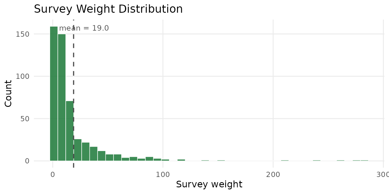
Distribution of survey weights. The right skew indicates that some providers represent many more population units than others.

Fitting the Weighted Model

Incorporating the survey design into hbb() requires three additional arguments — weights, stratum, and psu — each taking the name of the corresponding column in your data frame:

# This is the code you would run (takes ~2-5 minutes):
fit_w <- hbb(
  y | trials(n_trial) ~ poverty + urban,
  data    = nsece_synth_small,
  weights = "weight",
  stratum = "stratum",
  psu     = "psu",
  chains  = 4,
  seed    = 42
)

Behind the scenes, hbb() normalises the weights (so they sum to the sample size $N$ ), then multiplies each provider’s log-likelihood contribution by its weight. The result is a weighted pseudo-posterior that shifts point estimates toward the population-representative values.

results  <- readRDS(find_extdata("vig02_results.rds"))
sandwich <- readRDS(find_extdata("vig02_sandwich.rds"))
wald_ci  <- readRDS(find_extdata("vig02_wald_ci.rds"))
loo_comp <- readRDS(find_extdata("vig02_loo_compare.rds"))

cat(paste(results$print_text, collapse = "\n"))
#> Hurdle Beta-Binomial Model Fit
#> ==============================
#> 
#>   Model type   : Weighted (no random slopes, survey-weighted) 
#>   Stan model   : hbb_weighted 
#>   Formula      : y | trials(n_trial) ~ poverty + urban 
#> 
#>   Observations (N) : 504 
#>   Covariates   (P) : 3 (intercept + 2 predictors) 
#>   Zero rate        : 0.379 
#>   Survey weights   : yes 
#> 
#> MCMC:
#>   Chains           : 4 
#>   Warmup           : 1000 
#>   Sampling         : 1000 
#>   Total draws      : 4000 
#>   Elapsed          : 5.0 seconds 
#> 
#> Diagnostics:
#>   Divergent transitions : 0  [OK] 
#>   Max treedepth hits    : 0  [OK] 
#>   E-BFMI                : 1.105, 1.107, 1.028, 1.062 
#>   Max Rhat              : 1.0033  [OK] 
#>   Min bulk ESS          : 1946  [OK] 
#>   Min tail ESS          : 1951  [OK] 
#> 
#> Use summary() for parameter estimates.

Note the Weighted label — this confirms that survey weights were active during estimation.

The Pseudo-Posterior

In a standard Bayesian analysis the posterior is $\pi(\theta \mid y) \propto \pi(\theta) \prod_{i=1}^{N} L_i(\theta).$ The pseudo-log-likelihood replaces this with $\tilde{\ell}(\theta) = \sum_{i=1}^{N} \tilde{w}_i \, \log L_i(\theta),$ where $\tilde{w}_i = w_i / \bar{w}$ are the normalised weights. Providers representing more population units contribute proportionally more to the likelihood surface.

This is exactly what we want for point estimation: the posterior means target the finite-population parameters. However, the posterior standard deviations are no longer trustworthy for inference. The weights distort the curvature of the likelihood — a provider with weight 50 acts as though it were replicated 50 times, artificially inflating the effective sample size. The pseudo-posterior becomes too concentrated.

Key insight: the pseudo-posterior gives good point estimates but misleading uncertainty. We need the sandwich variance estimator to recover reliable standard errors.

Sandwich Standard Errors

The sandwich variance estimator has a long history in frequentist survey statistics. hurdlebb adapts it to the pseudo-posterior setting following Williams & Savitsky (2021):

$V_{\text{sand}} = H^{-1} \, J_{\text{cluster}} \, H^{-1}$

where:

$H$ is the observed Fisher information (the negative Hessian of the pseudo-log-posterior). Its inverse $H^{-1}$ is the “bread” — the variance you would get with a simple random sample.
$J_{\text{cluster}}$ is the clustered outer-product-of-gradients — the “meat” of the sandwich. It sums score contributions at the PSU level, capturing intra-cluster correlation.

One function call computes everything:

# In a live session:
sandwich <- sandwich_variance(fit_w)

The returned hbb_sandwich object contains the full matrix decomposition:

diag_df <- data.frame(
  parameter = sandwich$param_labels,
  H_inv     = round(diag(sandwich$H_obs_inv), 5),
  V_sand    = round(diag(sandwich$V_sand), 5)
)
diag_df$ratio <- round(diag_df$V_sand / diag_df$H_inv, 2)
diag_df
#>                           parameter   H_inv  V_sand ratio
#> alpha_(Intercept) alpha_(Intercept) 0.00891 0.06095  6.84
#> alpha_poverty         alpha_poverty 0.00783 0.03641  4.65
#> alpha_urban             alpha_urban 0.00354 0.00490  1.38
#> beta_(Intercept)   beta_(Intercept) 0.00288 0.01788  6.21
#> beta_poverty           beta_poverty 0.00219 0.00533  2.43
#> beta_urban               beta_urban 0.00211 0.00551  2.61
#> log_kappa                 log_kappa 0.00676 0.00790  1.17

The ratio column is the design effect ratio (DER), which we examine next.

Design Effect Ratios

The design effect ratio (DER) quantifies how much the survey design inflates each parameter’s variance relative to a simple random sample:

$\text{DER}_p = \frac{V_{\text{sand},pp}}{H^{-1}_{pp}}.$

A DER of 1.0 means the survey design has no impact. A DER of 5.0 means the true variance is five times larger than a naive analysis would suggest — equivalently, the naive standard error is $\sqrt{5} \approx 2.24$ times too small.

der_df <- data.frame(
  parameter = sandwich$param_labels,
  DER       = round(sandwich$DER, 2),
  SE_ratio  = round(sqrt(sandwich$DER), 2)
)
knitr::kable(der_df, align = c("l", "r", "r"),
             caption = "Design effect ratios by parameter.")

Design effect ratios by parameter.
	parameter	DER	SE_ratio
alpha_(Intercept)	alpha_(Intercept)	6.84	2.62
alpha_poverty	alpha_poverty	4.65	2.16
alpha_urban	alpha_urban	1.38	1.18
beta_(Intercept)	beta_(Intercept)	6.22	2.49
beta_poverty	beta_poverty	2.43	1.56
beta_urban	beta_urban	2.61	1.61
log_kappa	log_kappa	1.17	1.08

if (requireNamespace("ggplot2", quietly = TRUE)) {
  library(ggplot2)
  der_plot <- data.frame(
    parameter = factor(sandwich$param_labels,
                       levels = sandwich$param_labels[order(sandwich$DER)]),
    DER       = sandwich$DER,
    margin    = ifelse(grepl("^alpha", sandwich$param_labels), "Extensive",
                ifelse(grepl("^beta",  sandwich$param_labels), "Intensive",
                       "Dispersion"))
  )
  der_plot$margin <- factor(der_plot$margin,
                            levels = c("Extensive", "Intensive", "Dispersion"))

  ggplot(der_plot, aes(x = DER, y = parameter, fill = margin)) +
    geom_col(alpha = 0.85, width = 0.65) +
    geom_vline(xintercept = 1, linetype = "dashed", colour = "grey40",
               linewidth = 0.6) +
    geom_text(aes(label = sprintf("%.2f", DER)),
              hjust = -0.15, size = 3.3, colour = "grey20") +
    scale_fill_manual(
      values = c(Extensive = pal["extensive"], Intensive = pal["intensive"],
                 Dispersion = pal["dispersion"]),
      name = "Margin"
    ) +
    scale_x_continuous(expand = expansion(mult = c(0, 0.15))) +
    labs(x = "Design Effect Ratio (DER)", y = NULL,
         title = "Design Effect Ratios") +
    theme_minimal(base_size = 12) +
    theme(panel.grid.major.y = element_blank(),
          panel.grid.minor = element_blank(),
          legend.position = "bottom")
}
#> Warning: No shared levels found between `names(values)` of the manual scale and the
#> data's fill values.
#> No shared levels found between `names(values)` of the manual scale and the
#> data's fill values.
#> No shared levels found between `names(values)` of the manual scale and the
#> data's fill values.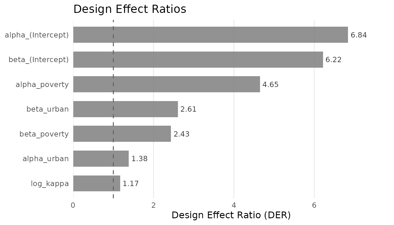

Design effect ratios (DER) by parameter. The dashed line at DER = 1 marks no design effect. Intercepts show the greatest inflation; the dispersion parameter is largely unaffected.

Several patterns are worth noting:

Intercepts have the largest DERs (6.84 for extensive, 6.22 for intensive). This is common: the overall mean is most sensitive to clustering because every unit within a cluster shares the same local baseline.
Slope coefficients have moderate DERs (1.38 to 4.65). Within-cluster variation in covariates partially offsets the clustering effect.
The dispersion parameter ( $\log\kappa$ ) has the smallest DER (1.17), because overdispersion is driven by within-unit variability, not clustering.

The mean DER across all seven parameters is 3.62. As a guideline: DERs above 2–3 indicate that ignoring the survey design would lead to materially overconfident inference.

Posterior vs. Wald Confidence Intervals

We can now contrast two types of intervals:

Posterior intervals (from the pseudo-posterior MCMC draws). These are too narrow because they do not account for the survey design.
Wald intervals constructed as $\hat\theta_p \pm z_{0.975} \times \text{SE}_{\text{sand},p}$ . These are design-consistent.

The summary() method accepts a sandwich argument to produce the Wald version. Compare the two:

cat("=== Posterior inference ===\n")
#> === Posterior inference ===
cat(paste(results$summary_text, collapse = "\n"))
#> 
#> ============================================================ 
#>   Hurdle Beta-Binomial Model Summary
#> ============================================================ 
#> 
#>   Model type   : Weighted (survey-weighted) 
#>   Formula      : y | trials(n_trial) ~ poverty + urban 
#>   Observations : 504 
#>   Zero rate    : 37.9% 
#>   Inference    : Posterior (MCMC)
#>   Level        : 0.95 
#> 
#> -------------------------------------------------- 
#>   Extensive Margin (alpha)
#> -------------------------------------------------- 
#>   Parameter          Estimate     SE  CI_lower  CI_upper    Rhat   ESS
#>   alpha_(Intercept)     0.321  0.096     0.133     0.505  1.0016  4633
#>   alpha_poverty        -0.059  0.089    -0.238     0.113  1.0006  4269
#>   alpha_urban           0.037  0.060    -0.079     0.152  1.0016  4239
#> 
#> -------------------------------------------------- 
#>   Intensive Margin (beta)
#> -------------------------------------------------- 
#>   Parameter         Estimate     SE  CI_lower  CI_upper    Rhat   ESS
#>   beta_(Intercept)    -0.074  0.048    -0.167     0.021  1.0020  5016
#>   beta_poverty         0.034  0.047    -0.059     0.128  1.0005  4987
#>   beta_urban          -0.005  0.032    -0.068     0.056  1.0006  4431
#> 
#> -------------------------------------------------- 
#>   Dispersion
#> -------------------------------------------------- 
#>   kappa = 6.840 (log_kappa = 1.923, SE = 0.097)
#>   kappa 95% CI: [5.618, 8.224]
#> 
#> -------------------------------------------------- 
#>   MCMC Diagnostics
#> -------------------------------------------------- 
#>   Divergent transitions    : 0 [OK]
#>   Max treedepth hits       : 0 [OK]
#>   E-BFMI                   : 1.105, 1.107, 1.028, 1.062 [OK]
#>   Max Rhat                 : 1.003 [OK]
#>   Min ESS (bulk)           : 1946 [OK]
#>   Min ESS (tail)           : 1951 [OK]

cat("=== Wald inference (sandwich SE) ===\n")
#> === Wald inference (sandwich SE) ===
cat(paste(results$summary_wald_text, collapse = "\n"))
#> 
#> ============================================================ 
#>   Hurdle Beta-Binomial Model Summary
#> ============================================================ 
#> 
#>   Model type   : Weighted (survey-weighted) 
#>   Formula      : y | trials(n_trial) ~ poverty + urban 
#>   Observations : 504 
#>   Zero rate    : 37.9% 
#>   Inference    : Wald (sandwich SE)
#>   Level        : 0.95 
#> 
#> -------------------------------------------------- 
#>   Extensive Margin (alpha)
#> -------------------------------------------------- 
#>   Parameter          Estimate     SE  CI_lower  CI_upper    Rhat   ESS
#>   alpha_(Intercept)     0.321  0.247    -0.163     0.805  1.0016  4633
#>   alpha_poverty        -0.059  0.191    -0.433     0.315  1.0006  4269
#>   alpha_urban           0.037  0.070    -0.100     0.175  1.0016  4239
#> 
#> -------------------------------------------------- 
#>   Intensive Margin (beta)
#> -------------------------------------------------- 
#>   Parameter         Estimate     SE  CI_lower  CI_upper    Rhat   ESS
#>   beta_(Intercept)    -0.074  0.134    -0.336     0.188  1.0020  5016
#>   beta_poverty         0.034  0.073    -0.109     0.177  1.0005  4987
#>   beta_urban          -0.005  0.074    -0.150     0.141  1.0006  4431
#> 
#> -------------------------------------------------- 
#>   Dispersion
#> -------------------------------------------------- 
#>   kappa = 6.840 (log_kappa = 1.923, SE = 0.089)
#>   kappa 95% CI: [5.746, 8.141]
#> 
#> -------------------------------------------------- 
#>   MCMC Diagnostics
#> -------------------------------------------------- 
#>   Divergent transitions    : 0 [OK]
#>   Max treedepth hits       : 0 [OK]
#>   E-BFMI                   : 1.105, 1.107, 1.028, 1.062 [OK]
#>   Max Rhat                 : 1.003 [OK]
#>   Min ESS (bulk)           : 1946 [OK]
#>   Min ESS (tail)           : 1951 [OK]
#> 
#> -------------------------------------------------- 
#>   Design Effect Ratios (DER)
#> -------------------------------------------------- 
#>   alpha_(Intercept)          6.842
#>   alpha_poverty              4.651
#>   alpha_urban                1.385
#>   beta_(Intercept)           6.218
#>   beta_poverty               2.434
#>   beta_urban                 2.606
#>   log_kappa                  1.168
#> 
#>   DER range: [1.168, 6.842], mean: 3.615

The Wald CI table from compute_wald_ci():

knitr::kable(
  wald_ci[, c("parameter", "post_mean", "se", "z_stat",
              "p_value", "ci_lo", "ci_hi", "significant")],
  digits = 3, align = c("l", rep("r", 7)),
  caption = "Wald 95% confidence intervals from sandwich variance."
)

Wald 95% confidence intervals from sandwich variance.
parameter	post_mean	se	z_stat	p_value	ci_lo	ci_hi	significant
alpha_(Intercept)	0.321	0.247	1.300	0.194	-0.163	0.805	FALSE
alpha_poverty	-0.059	0.191	-0.308	0.758	-0.433	0.315	FALSE
alpha_urban	0.037	0.070	0.535	0.593	-0.100	0.175	FALSE
beta_(Intercept)	-0.074	0.134	-0.552	0.581	-0.336	0.188	FALSE
beta_poverty	0.034	0.073	0.464	0.642	-0.109	0.177	FALSE
beta_urban	-0.005	0.074	-0.063	0.950	-0.150	0.141	FALSE
log_kappa	1.923	0.089	21.635	0.000	1.749	2.097	TRUE

The forest plot below makes the comparison visual. For each parameter, the thin line shows the posterior credible interval and the thick translucent line shows the wider Wald confidence interval:

if (requireNamespace("ggplot2", quietly = TRUE)) {
  library(ggplot2)

  post_fe <- results$summary_obj$fixed_effects
  wald_fe <- results$summary_wald_obj$fixed_effects

  ci_df <- data.frame(
    parameter  = post_fe$parameter,
    estimate   = post_fe$estimate,
    post_lo    = post_fe$ci_lower,
    post_hi    = post_fe$ci_upper,
    wald_lo    = wald_fe$ci_lower,
    wald_hi    = wald_fe$ci_upper,
    margin     = ifelse(grepl("^alpha", post_fe$parameter), "Extensive",
                 ifelse(grepl("^beta",  post_fe$parameter), "Intensive",
                        "Dispersion")),
    stringsAsFactors = FALSE
  )
  ci_df$margin <- factor(ci_df$margin,
                         levels = c("Extensive", "Intensive", "Dispersion"))
  ci_df$ypos <- rev(seq_len(nrow(ci_df)))

  margin_col <- c(Extensive = pal["extensive"], Intensive = pal["intensive"],
                  Dispersion = pal["dispersion"])

  ggplot(ci_df) +
    # Wald CI (thick, behind)
    geom_segment(aes(x = wald_lo, xend = wald_hi,
                     y = ypos - 0.12, yend = ypos - 0.12,
                     colour = margin),
                 linewidth = 3, alpha = 0.3) +
    geom_point(aes(x = estimate, y = ypos - 0.12, colour = margin),
               shape = 17, size = 2.5) +
    # Posterior CI (thin, in front)
    geom_segment(aes(x = post_lo, xend = post_hi,
                     y = ypos + 0.12, yend = ypos + 0.12,
                     colour = margin),
                 linewidth = 0.9) +
    geom_point(aes(x = estimate, y = ypos + 0.12, colour = margin),
               shape = 1, size = 2.5, stroke = 0.8) +
    # Zero reference
    geom_vline(xintercept = 0, linetype = "dashed", colour = "grey50",
               linewidth = 0.5) +
    scale_colour_manual(values = margin_col, name = "Margin") +
    scale_y_continuous(breaks = ci_df$ypos, labels = ci_df$parameter) +
    labs(x = "Estimate (95% interval)", y = NULL,
         title = "Posterior vs. Wald Confidence Intervals",
         subtitle = "Open circles / thin = Posterior;  Filled triangles / thick = Wald") +
    theme_minimal(base_size = 12) +
    theme(legend.position = "bottom",
          panel.grid.major.y = element_blank(),
          panel.grid.minor = element_blank(),
          plot.subtitle = element_text(size = 9, colour = "grey40"))
}
#> Warning: No shared levels found between `names(values)` of the manual scale and the
#> data's colour values.
#> No shared levels found between `names(values)` of the manual scale and the
#> data's colour values.
#> No shared levels found between `names(values)` of the manual scale and the
#> data's colour values.
#> No shared levels found between `names(values)` of the manual scale and the
#> data's colour values.
#> No shared levels found between `names(values)` of the manual scale and the
#> data's colour values.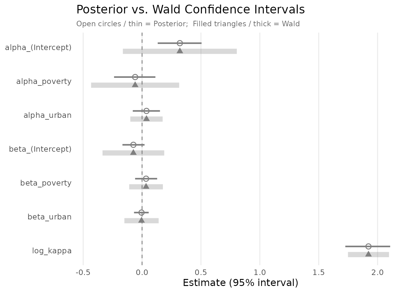

Forest plot comparing posterior (thin lines, open circles) and Wald (thick translucent lines, filled triangles) 95% intervals. Wald intervals are consistently wider, reflecting the true sampling variability from the complex survey design.

The pattern is striking. For alpha_poverty, the posterior standard error is 0.089 while the sandwich standard error is 0.191 — more than twice as large, consistent with a DER of 4.65 ( $\sqrt{4.65} \approx 2.16$ ). Using the posterior interval alone, you might conclude that poverty has a statistically significant negative effect on participation. The Wald interval, which properly accounts for the survey design, is much wider and includes zero.

CI Width Comparison

A grouped bar chart makes the inflation tangible:

if (requireNamespace("ggplot2", quietly = TRUE)) {
  library(ggplot2)

  post_fe <- results$summary_obj$fixed_effects
  wald_fe <- results$summary_wald_obj$fixed_effects

  width_df <- data.frame(
    parameter  = post_fe$parameter,
    post_width = post_fe$ci_upper - post_fe$ci_lower,
    wald_width = wald_fe$ci_upper - wald_fe$ci_lower,
    stringsAsFactors = FALSE
  )
  width_df$ratio <- round(width_df$wald_width / width_df$post_width, 2)

  width_long <- rbind(
    data.frame(parameter = width_df$parameter,
               width = width_df$post_width, type = "Posterior"),
    data.frame(parameter = width_df$parameter,
               width = width_df$wald_width, type = "Wald (sandwich)")
  )
  width_long$parameter <- factor(width_long$parameter,
                                 levels = width_df$parameter)
  width_long$type <- factor(width_long$type,
                            levels = c("Posterior", "Wald (sandwich)"))

  ggplot(width_long, aes(x = parameter, y = width, fill = type)) +
    geom_col(position = position_dodge(width = 0.7), width = 0.6) +
    geom_text(data = width_df,
              aes(x = parameter, y = wald_width,
                  label = paste0(ratio, "x")),
              inherit.aes = FALSE,
              vjust = -0.5, size = 3, colour = "grey30") +
    scale_fill_manual(
      values = c("Posterior" = pal["extensive"],
                 "Wald (sandwich)" = pal["intensive"]),
      name = NULL
    ) +
    labs(x = NULL, y = "95% CI Width",
         title = "Posterior vs. Wald Interval Widths") +
    theme_minimal(base_size = 12) +
    theme(axis.text.x = element_text(angle = 30, hjust = 1),
          legend.position = "top",
          panel.grid.minor = element_blank())
}
#> Warning: No shared levels found between `names(values)` of the manual scale and the
#> data's fill values.
#> No shared levels found between `names(values)` of the manual scale and the
#> data's fill values.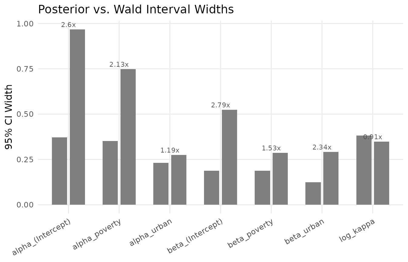

CI width comparison. Wald intervals (red) are uniformly wider than posterior intervals (blue). The ratio printed above each pair approximates the square root of the DER.

Model Comparison with LOO

You may wonder whether the weighted model fits better than the unweighted version. LOO-CV provides the comparison:

# In a live session:
loo_comp <- hbb_loo_compare(base = fit_base, weighted = fit_w)

cat("Model comparison:\n")
#> Model comparison:
print(loo_comp$comparison[, c("model", "elpd_loo", "elpd_diff", "se_diff")])
#>      model  elpd_loo elpd_diff  se_diff
#> 1     base -1485.788   0.00000 0.000000
#> 2 weighted -1496.856 -11.06773 5.800007
cat("\nPairwise z-ratio:\n")
#> 
#> Pairwise z-ratio:
print(loo_comp$pairwise)
#>         comparison delta_elpd  se_diff  z_ratio
#> 1 base vs weighted   11.06773 5.800007 1.908227

The base (unweighted) model has a slightly higher ELPD ( $-1485.8$ ) than the weighted model ( $-1496.9$ ), with a difference of $11.07$ and $z = 1.91$ . This difference is not significant at conventional levels.

This result may seem counterintuitive — if weights improve inference, why does the weighted model predict less well? The answer lies in what LOO measures. LOO evaluates predictive accuracy for the sample at hand, not population inference. The survey weights distort the likelihood to target population parameters, which can reduce in-sample predictive performance. This is expected behaviour.

Guideline: Do not use LOO to choose between weighted and unweighted models. The decision should be driven by your inferential goal: if the data come from a complex survey and you want population-level conclusions, use weights.

Complete Workflow Summary

Putting it all together:

# 1. Fit weighted model
fit <- hbb(
  y | trials(n_trial) ~ poverty + urban,
  data = nsece_synth_small,
  weights = "weight", stratum = "stratum", psu = "psu",
  chains = 4, seed = 42
)

# 2. Posterior summary (naive SEs --- useful for MCMC diagnostics)
summary(fit)

# 3. Sandwich variance (design-corrected SEs)
sand <- sandwich_variance(fit)

# 4. Wald summary (design-corrected CIs + DER)
summary(fit, sandwich = sand)

# 5. Explicit Wald CI table
wald <- compute_wald_ci(coef(fit), sand$V_sand, level = 0.95)

When to Use Corrections

Situation	Recommendation
Simple random sample	Use unweighted `hbb()`, posterior CIs
Stratified design, no clustering	Weights may suffice; check DER
Stratified clustered design	Full pipeline: weights + sandwich + Wald CIs
DER $< 1.2$ for all parameters	Posterior CIs are adequate
DER $> 2$ for key parameters	Sandwich-based Wald CIs are essential

Reporting. In your manuscript, report posterior means as point estimates and Wald confidence intervals as the uncertainty measure. Include the DER table in a supplement so readers can gauge the severity of design effects.

What’s Next?

Vignette	What you will learn
State-Varying Coefficients	Hierarchical model with state-level random slopes + survey weights
Policy Moderators	Cross-level interactions explaining state variation
Marginal Effects	AME decomposition with design-corrected standard errors

JoonHo Lee

2026-04-21