Chapter 8 made one claim repeatedly: a reliability coefficient is a functional of the design and the population, every coefficient in circulation is the same ratio with different estimates plugged in, and the choice among them matters exactly as much as information varies over the population. Under the Rasch model that variation is bounded, because items differ only in placement, and the chapter could treat the disagreements among functionals as a caution. Under the 2PL the caution becomes the story. Discrimination heterogeneity is precisely a machine for making information uneven (Chapter 24), and uneven information is precisely the condition under which the members of the reliability zoo part company.
This chapter states the mechanism and shows it in a stylized pair of tests. It then asks how two operational catalogue coefficients move across thirteen real tests, without treating that catalogue as a same-fit demonstration of the stylized mechanism, and records two facts about the reliability ladder that the evidence chapters depend on.
The zoo, revisited where it bites
Recall the two population functionals of Equation 8.13: the MSEM form \(\bar\rho\), which averages error variance \(1/\mathcal{J}(\theta)\) over \(G\) and then forms the ratio, and the average-information form \(\tilde\rho\), which averages \(\mathcal{J}\) first. Theorem 8.1 orders them, \(\tilde\rho \ge \bar\rho\), with equality only when information is constant over the population. A Rasch test can hold the gap modest. A 2PL test with concentrated discriminations drives it wide, because \(1/\mathcal{J}\) explodes in the information deserts that concentration creates while \(\operatorname{E}[\mathcal{J}]\) barely notices them.
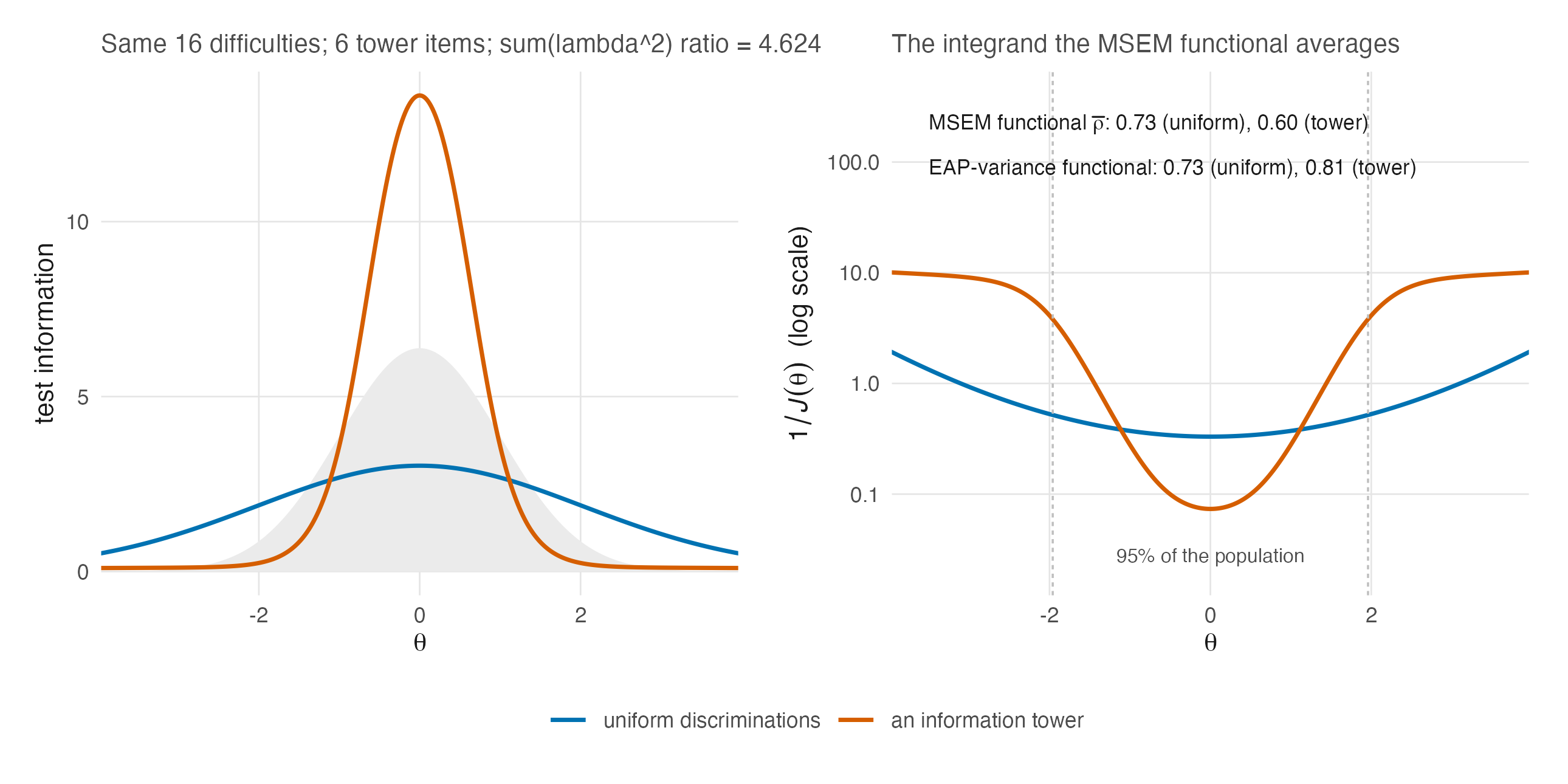
Alongside these sits the EAP-variance form, the variance of the posterior means relative to the trait variance (Section 8.6). It is computed from realized posteriors. It should not be conflated with every coefficient that fitted software calls “marginal reliability”: in particular, mirt::marginal_rxx integrates a pointwise information ratio and does not compute the variance of EAPs or average posterior variances. A test that concentrates information under the population mass can nevertheless score well by the EAP-variance functional while scoring badly by the MSEM functional, and the two can move in opposite directions when the model family changes.
Figure 25.1 exhibits the mechanism in its pure form: two sixteen-item tests with identical difficulties, one uniform, one an information tower, for which the MSEM functional prefers the uniform test by a wide margin while the EAP-variance functional prefers the tower.
Neither functional is wrong. Both average with respect to a population \(G\), but they assemble uncertainty differently: \(\bar\rho\) first uses inverse information as an error-variance approximation, whereas the EAP-variance form uses the spread of the exact posterior means under the fitted scoring model. The 2PL manufactures designs for which those operations give different answers. The practical rule this book keeps returning to gains a clause: a reliability number needs its coefficient named, and under the 2PL it also needs the model family named, because the family is part of what the coefficient is measuring.
Thirteen real tests, two catalogue summaries each
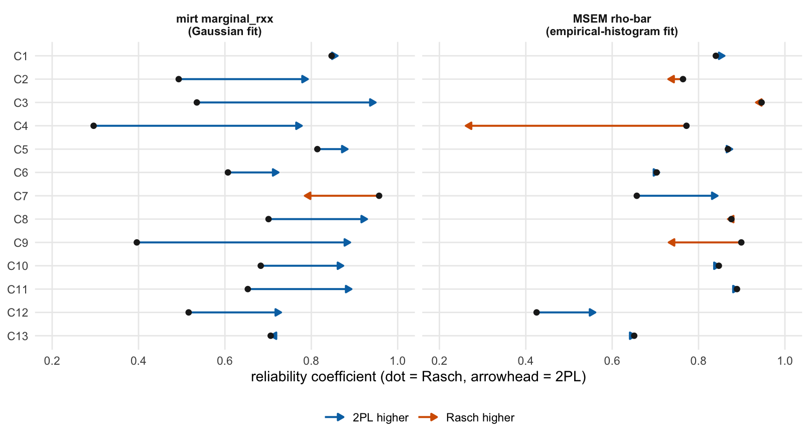
The case-study volume fitted every one of its thirteen Item Response Warehouse cases under both item models and placed two coefficients beside each other (Lee 2026b). The first is mirt::marginal_rxx from the Gaussian mirt fit, an information-ratio coefficient rather than a posterior-variance or EAP-variance coefficient. The second is the MSEM functional \(\bar\rho\) of Equation 8.13, evaluated from the separate empirical-histogram fit. The two columns use the same response matrix within a case, but not the same fitted object or the same functional. Figure 25.2 displays the full descriptive catalogue, and Table 25.1 carries the values.
Two features deserve the reader’s pause. The first is how often the arrows disagree: the two catalogue columns agree about the direction of the item-model change in only six of the thirteen cases. At the portfolio level the median Rasch-to-2PL gap is \(+0.215\) for mirt::marginal_rxx against \(+0.004\) for the empirical-histogram MSEM functional. Those medians describe the catalogue; they do not isolate a coefficient effect because the fitted population model changes with the column. The second feature is case C4, a sixteen-item vocabulary checklist administered alongside a conspiracist-belief scale. Its Gaussian-fit mirt::marginal_rxx rises from .30 to .78 when the 2PL replaces the Rasch model, while the empirical-histogram MSEM functional falls from .77 to .26. The responses are the same, but the coefficient and fitted object are not. The magnitude makes the discrepancy important; it does not by itself show that the information-tower mechanism in Figure 25.1 caused it. Establishing that claim would require evaluating both target functionals on the same fitted item parameters and the same \(G\).
The lesson is not that one column of Table 25.1 is the true reliability. It is that “is the 2PL more reliable than the Rasch model here?” is not a well-posed question until the coefficient, fitted population model, and averaging distribution are named. That is Chapter 8’s claim returned with real data attached; the present catalogue does not separate those ingredients.
The corpus-scale version of the same lesson comes from the reliability study of the Item Response Warehouse, whose complete analysis corpus contains 889 datasets. Across six estimators its reported pooled coefficients span .794 to .868, and its estimated share below the .80 convention runs from roughly a quarter to a half (Lee 2026c). The complete 889-row per-unit snapshot used by this book’s evidence pipeline is a frozen analysis artifact, not the public replication frame: the latter contains 879 rows because ten datasets are withheld. The quoted span and sub-.80 range are the manuscript’s full-corpus results, not a recomputation from the public 879-row file. Chapter 28 takes up the study properly; here the result shows that definition-sensitive reliability is not confined to one small case portfolio.
What the simulation’s ladder actually manipulated
The evidence chapters read results off a design in which reliability is a manipulated factor, so this book must say precisely what the manipulation was. Two facts matter, and both are read from the simulation volume’s frozen design tables rather than from its prose (Lee 2026a).
The operational coefficient is the information approximation. The ladder targets \(\bar\rho\) in the form \(\sigma^2_\theta / \{\sigma^2_\theta + \operatorname{E}_G[1/\mathcal{J}(\theta)]\}\) — the population MSEM functional of Equation 8.10 with information standing in for estimator error variance. Chapter 7 was explicit that information omits calibration uncertainty and model error, and Proposition 7.1 separates this average from its companion; the ladder’s “reliability” is therefore a specific, computable functional, not a claim about any realized coefficient a fitted run would report. The distinction did no harm in the design, since achieved and target values agree to three decimals, but a reader who carries Chapter 8’s vocabulary should know which member of the zoo the design axis is.
The instrument was length and a discrimination multiplier. Each cell of the ladder was calibrated by choosing a test length and, jointly, a global multiplier \(c^*\) applied to the form’s discriminations: the scale lever of Section 9.3 and Proposition 9.1, exercised in production. Table 25.2 displays the realized ladder with the multiplier column intact.
The multipliers are not decoration: they range over roughly 0.79 to 1.09 across cells, and they are how the calibration hit its targets to within 0.003 at every tier. The consequence for interpretation is the one Section 9.4 already taught for the manuscript’s own Table 2, now applied to the companion study: reliability was set through the design, so the ladder’s axis is a bundle, length and discrimination scale moving together, and any statement of the form “the effect of reliability” is a statement about that bundle. The simulation volume’s own regression diagnostic makes the entanglement concrete: achieved reliability and log test length correlate at .98 across its estimation rows, and a model asking the two to speak separately returns a variance inflation factor above thirty (Lee 2026a). Nothing is wrong with the bundle as a design; things would be wrong with reading it as a partial derivative. The open design that would separate the levers, varying discrimination at fixed length, is recorded as unfinished business in Chapter 29.
Sources and provenance
The two population functionals, their Jensen ordering, the EAP-variance coefficient, and the source reading of mirt::marginal_rxx are Chapter 8’s; nothing in Section 25.1 modifies them. Figure 25.1 is computed for this chapter (exact quadrature for \(\bar\rho\); a seeded 4,000-person computation for the EAP-variance functional; values frozen in tables/F-rel-functionals-summary.rds) and its design is stylized, chosen to show that reversal is possible rather than to reproduce any case-study fit.
Table 25.1 and Figure 25.2 are read from the case-study analysis layer’s frozen P1-T2 catalogue (Lee 2026b). The citation names the second edition, which added no fits and recomputed no frozen values; this book reads the P1-T2 table from the first-edition repository. Its left column calls mirt::marginal_rxx(fp$gauss); its right column evaluates rho_bar_eh from fp$eh. Thus response data and item-model label are matched, while fitted object and functional differ. The C4 values quoted in prose are asserted against that table by the build before either display is written. The corpus span .794 to .868 and the definition-dependent sub-.80 shares are the Item Response Warehouse reliability study’s full-889-dataset manuscript results (Lee 2026c), read from manuscript v3 dated 2026-08-06. The evidence pipeline’s complete 889-row snapshot is distinct from the public 879-row replication frame; Chapter 28 gives the study design and fuller provenance.
The ladder facts are the simulation volume’s frozen rollup, surfaced here as Table 25.2 with the same assertions (Lee 2026a); the correlation .98 and the variance inflation factor are that volume’s own published diagnostics, quoted as published. The reading of the ladder as a bundle is this book’s, and is the same reading Section 9.4 gave the manuscript’s design; the underlying scale-lever result is Proposition 9.1, restated from the reliability-targeting package (Lee 2026d), whose companion paper develops the calibration algorithms themselves (Lee 2026e).
Lee, JoonHo. 2026a.
A Simulation Study of Dirichlet Process Mixture Priors and Goal-Specific Posterior Summaries in Bayesian IRT. Quarto book, The University of Alabama.
https://joonho112.github.io/dpmirt-simulation-study/.
Lee, JoonHo. 2026b.
Case Studies of Dirichlet Process Mixture Priors and Goal-Specific Posterior Summaries in Bayesian IRT: Thirteen Real Tests from the Item Response Warehouse. Quarto book, The University of Alabama.
https://joonho112.github.io/dpmirt-case-studies/.
Lee, JoonHo. 2026c.
How Reliable Are Psychological Measurements? The Distribution of Marginal Reliability Across 889 Item-Response Datasets.
arXiv; arXiv.
https://doi.org/10.48550/arXiv.2608.06806.
Lee, JoonHo. 2026d.
IRTsimrel: Reliability-Targeted Simulation for Item Response Data.
https://github.com/joonho112/IRTsimrel.
Lee, JoonHo. 2026e.
Reliability-Targeted Simulation of Item Response Data: Solving the Inverse Design Problem.
arXiv; arXiv.
https://doi.org/10.48550/arXiv.2512.16012.