This article runs cacs_run() for one example site and
explains the table it returns. Its calculations use only data installed
with the package, so they run without a Census API key or an internet
connection.
What catchmentACS does
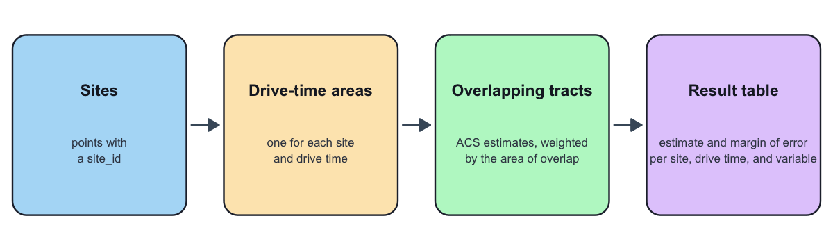
For each site and each drive time, such as 5, 10, and 15 minutes, catchmentACS finds the area that can be reached by car within that time, called the drive-time area or isochrone. It then combines the American Community Survey (ACS) estimates of the census tracts that overlap the area into estimates for the area, such as the number of people below the poverty level. Each estimate comes with a margin of error, the half-width of its 90 percent confidence interval.
When a tract lies partly inside the area, its counts are included in proportion to the share of the tract’s area that lies inside, which assumes that people and households are spread evenly within the tract. The medians and per-person values of three ACS tables (median household income, median home value, and per capita income) are averaged over the tracts instead, with weights proportional to the area each tract shares with the drive-time area. The average stands in for the median or per-person value of the drive-time area. Its weights ignore how many people live in each tract, so it can be far from that value when the tracts differ in population density. A median or per-person value from any other table is added up like a count.
cacs_run() does all of this in one call and returns a
table with one row for each site, drive time, and variable. The
calculations are described in
vignette("methodology", package = "catchmentACS").
Install
When catchmentACS is available on CRAN,
install.packages("catchmentACS") installs the released
version. The development version is on GitHub:
# install.packages("pak")
pak::pak("joonho112/catchmentACS")
A version installed from CRAN includes the package’s articles, such
as this one; a version installed from GitHub with
pak::pak() does not. The articles are also on the package
website, https://joonho112.github.io/catchmentACS/articles/.
Building drive-time areas with the default routing service needs the
osrm package, and the package’s maps need the leaflet package. Neither
is installed with catchmentACS:
install.packages(c("osrm", "leaflet"))Downloading ACS data requires a free Census API key, which you can
request at https://api.census.gov/data/key_signup.html. The
following call saves the key in your .Renviron file; it
takes effect after R is restarted or after
readRenviron("~/.Renviron"):
tidycensus::census_api_key("YOUR_KEY_HERE", install = TRUE)The default routing service is the Open Source Routing Machine (OSRM), used through a public server that does not need a key.
A first run on the example data
The example reads three files installed with the package. They hold
made-up data: 20 sites on a grid over a rectangle around Alabama,
drive-time areas drawn as circles around the sites, and random ACS
estimates for 911 small squares, spaced apart, that serve as census
tracts. Given the areas and the estimates, cacs_run() skips
the steps that build the areas and download the estimates. The example
uses the site AL_SITE_07 and its areas for drive times of
5, 10, and 15 minutes.
# Load the three bundled example inputs.
sites <- readRDS(system.file(
  "extdata", "legacy_2025_sites.rds", package = "catchmentACS"
))
iso <- readRDS(system.file(
  "extdata", "legacy_2025_isochrones.rds", package = "catchmentACS"
))
acs <- readRDS(system.file(
  "extdata", "sample_alabama_subset.rds", package = "catchmentACS"
))

one_site <- "AL_SITE_07"

result <- cacs_run(
  sites                  = sites[sites$site_id == one_site, , drop = FALSE],
  state                  = "AL",
  precomputed_isochrones = iso[iso$site_id == one_site, , drop = FALSE],
  acs                    = acs,
  verbose                = FALSE
)

dim(result)
#> [1] 57 27The arguments of the call:
-
sites: the sites, as a data frame with the columnssite_id,lon, andlat, or as an sf object of points with asite_idcolumn, like the example sites. -
state: the state whose tracts are downloaded. -
precomputed_isochronesandacs: drive-time areas and ACS estimates that are already at hand, in the forms thatcacs_isochrone()andcacs_acs_prefetch()return. -
verbose:FALSEturns off the messages that report which steps run and how they progress.
The other arguments keep their defaults, such as the 2019–2023 ACS
5-year estimates (year = 2023), drive times of 5, 10, and
15 minutes, OSRM as the routing service, area weighting, and the long
format of the result. ?cacs_run describes every
argument.
With both precomputed_isochrones and acs
supplied, cacs_run() uses every area in
precomputed_isochrones and every variable in
acs, so the example selects the areas of
AL_SITE_07 itself. sites,
drive_times, and provider are then only
recorded with the result and shown when it is printed;
state and year are only recorded.
For your own sites, the call is the same without
precomputed_isochrones and acs. It then needs
the osrm package, the Census API key described under Install, and an
internet connection, so the call below is not run here.
vignette("providers", package = "catchmentACS") describes
the routing services and the API keys. The call uses the sites
cacs_alabama_sites, ten made-up points near the centers of
Alabama cities. They reuse the site_id values of the
example data for other places: their AL_SITE_07 is not the
site used above.
result_live <- cacs_run(
  sites       = cacs_alabama_sites,   # or your own sites
  state       = "AL",
  year        = 2023,
  drive_times = c(5, 10, 15),
  provider    = "osrm",
  output      = "long"
)
vignette("alabama-tutorial", package = "catchmentACS")
goes through the steps of cacs_run() one at a time on the
same example data and turns the result into tables for a report.
Reading the result
result has 57 rows: the 14 ACS variables and the five
rates for each of the three drive times. Besides the estimates and their
margins of error, its columns record how each row was computed, such as
the weights and the formula for the margin of error;
?cacs_run describes them all.
The rows for the 15-minute area, with the columns discussed below:
rows_15 <- tibble::as_tibble(result) |>
  filter(drive_time_min == 15) |>
  select(variable, estimate, moe, failure_origin)
rows_15
#> # A tibble: 19 × 4
#> variable estimate moe failure_origin
#> <chr> <dbl> <dbl> <chr>
#> 1 B01003_001 11481 1195. none
#> 2 B11001_001 5046 370. none
#> 3 B17001_001 8364 869. none
#> 4 B17001_002 3010 241. none
#> 5 B19013_001 60498. 7834. none
#> 6 B19056_001 3444 274. none
#> 7 B19056_002 426 47.2 none
#> 8 B19301_001 25135. 2643. none
#> 9 B22003_001 4634 386. none
#> 10 B22003_002 516 35.2 none
#> 11 B23025_001 6850 532. none
#> 12 B23025_002 4974 530. none
#> 13 B23025_003 4979 353. none
#> 14 B23025_005 459 48.7 none
#> 15 poverty_rate 0.360 0.0472 none
#> 16 snap_rate 0.111 0.0120 none
#> 17 ssi_rate 0.124 0.0169 none
#> 18 unemp_rate 0.0922 0.0118 none
#> 19 labor_force_participation 0.726 0.0958 nonetibble::as_tibble() turns result into a
plain tibble, which keeps the rows in their order and prints without the
header and the rate tables that print() adds to a result of
cacs_run().
The first 14 rows are the ACS variables, named by their codes
(cacs_acs_default_vars gives each a short name). Most are
counts of people or households, such as the total population
(B01003_001); median household income
(B19013_001) and per capita income
(B19301_001) are averages, as described above. The last
five rows are the rates listed in cacs_acs_default_rates,
each the ratio of two of the counts. poverty_rate, for
example, divides the number of people below the poverty level
(B17001_002) by the number of people for whom poverty
status is determined (B17001_001).
vignette("theory-derived-rates", package = "catchmentACS")
describes the five rates and the formulas for their margins of
error.
moe is the margin of error at the 90 percent confidence
level, the default of cacs_run(): the estimate minus and
plus its margin of error are the ends of a 90 percent confidence
interval. For the poverty rate of the 15-minute area:
poverty_15 <- filter(rows_15, variable == "poverty_rate")
c(lower = poverty_15$estimate - poverty_15$moe,
  upper = poverty_15$estimate + poverty_15$moe)
#> lower upper
#> 0.3126909 0.4070605The estimated poverty rate is 36.0 percent, and its 90 percent confidence interval runs from 31.3 to 40.7 percent.
These margins of error treat the estimates of different tracts as
independent, and they leave out error from the area weighting and
uncertainty in the drive-time areas. If the tract estimates are
positively correlated, the margins of error of counts, medians, and
per-person values are too small. For a rate, such as the poverty rate
above, errors that move its numerator and denominator in the same
direction partly offset each other, and the package does not compute the
net effect.
vignette("theory-moe-propagation", package = "catchmentACS")
discusses these assumptions.
failure_origin names the step at which a row failed. It
is "isochrone" on every row, including the rates, of a site
and drive time for which the routing service returned no drive-time
area. It is "carrier" for a rate whose numerator or
denominator, or the margin of error of either, is missing. A site and
drive time with no tract left for its area has one row with
variable = NA and
failure_origin = "intersection" in place of the rows of the
ACS variables, and its rates are "carrier". Other rows have
"none". A missing tract estimate does not count as a
failure. When a tract in the area has no estimate for a variable, the
row for that variable has an NA estimate and
failure_origin = "none", even when only a small part of the
tract lies inside the area. The rates computed from that variable are
then NA with "carrier". This table crosses
failure_origin with missing estimates:
#>               missing_estimate
#> failure_origin FALSE
#>           none    57
In this example every row has an estimate. About 5 percent of the
tract estimates in the example data are missing, and other sites, such
as AL_SITE_04, have rows with NA estimates.
With another value of one_site, from
"AL_SITE_01" to "AL_SITE_20", the code in this
article gives the results and the map for that site. For most of the
other sites, cacs_run() also gives warnings, about rates
that are NA or about drive-time areas that reach beyond the
example ACS data.
summary() collects the five rates in a table with one
row for each site and drive time. Its element
rates_per_site_moe shows each rate with its margin of
error, rounded to three decimals:
#> # A tibble: 3 × 7
#>   site_id    drive_time_min poverty_rate  snap_rate     ssi_rate
#>   <chr>               <int> <chr>         <chr>         <chr>
#> 1 AL_SITE_07              5 0.618 ± 0.104 0.040 ± 0.006 0.167 ± 0.037
#> 2 AL_SITE_07             10 0.602 ± 0.098 0.043 ± 0.006 0.165 ± 0.036
#> 3 AL_SITE_07             15 0.360 ± 0.047 0.111 ± 0.012 0.124 ± 0.017
#>   unemp_rate    labor_force_participation
#>   <chr>         <chr>
#> 1 0.062 ± 0.015 0.851 ± 0.115
#> 2 0.063 ± 0.015 0.846 ± 0.112
#> 3 0.092 ± 0.012 0.726 ± 0.096
The rates for 5 and 10 minutes are close. The rows of any count show why:
tibble::as_tibble(result) |>
  filter(variable == "B01003_001") |>
  select(drive_time_min, estimate, moe, n_tracts, weight_sum)
#> # A tibble: 3 × 5
#> drive_time_min estimate moe n_tracts weight_sum
#> <int> <dbl> <dbl> <int> <dbl>
#> 1 5 4543 612 1 1
#> 2 10 4643. 612. 3 1.03
#> 3 15 11481 1195. 3 3n_tracts is the number of tracts combined, and
weight_sum adds up the share of each tract’s area that lies
inside the drive-time area. Here the 5-minute area covers one tract
whole, the 10-minute area adds small parts of two more, and the
15-minute area covers all three whole. Because each area contains the
shorter ones, the estimates for the three drive times are computed in
part from the same tract estimates and are not independent. The
Limitations section of
vignette("methodology", package = "catchmentACS") explains
what this means for comparing them.
A map of the drive-time areas
cacs_plot_site_isochrone() draws a site and its
drive-time areas on a web base map: the site as a red point and each
area in its own color, with a legend of the drive times. It needs the
leaflet package. In the example data, the three areas are circles
centered on the site, with radii of 5, 10, and 15 km.
padding_km = 20 makes the first view show at least 20 km on
each side of the site, so that all three fit:
cacs_plot_site_isochrone(
  site_id    = one_site,
  iso_sf     = iso,
  sites_df   = sites,
  padding_km = 20
)
Unlike these circles, an area built by a routing service follows the
road network.
vignette("visual-walkthrough", package = "catchmentACS")
draws this map for a site in Birmingham, Alabama, whose area was built
by OSRM, and three more maps, of the overlapping tracts, one ACS
variable, and the five rates.